A Castle Lookout Doesn’t Wait for Eye Colour: Why Climate Risk Needs a Better Standard of Evidence
Read this essay like a big adventure into a deeper understanding of the latest climate science . It has something for everyone, sceptic and believer, layman and scientist alike. Most of all, enjoy .

Climate Risk Needs a Better Standard of Evidence

Climate risk analysis has a core problem: its methods don’t reflect the risk.
We often ask for the kind of proof we would expect from a slow, stable, reversible system. But the climate isn’t that kind of system; it has feedback, thresholds, delays, and linked parts that can shift together. So it can change hardly at all, then all at once.
The issue is not that climate models are linear or that they ignore nonlinear physics. They do contain feedback, thresholds, turbulence, circulation dynamics, and abrupt responses.
The problem is that, to make the whole Earth computable, they must compress messy local processes into grid cells, parameterised rules, scenario choices, and ensemble summaries.
That compression is useful for estimating broad trends, but it can blur the features that matter most for risk: concentrated meltwater pulses, cloud-regime shifts, abrupt weakening of circulation, ecological tipping points, and correlated failure modes.
In practice, the modelling workflow can make dangerous changes appear smoother, slower, and more geographically averaged than the physical system may be. So the failure is not that models are useless; it is that model architecture and reporting conventions can under-resolve the sharp edges of risk, especially when society mistakes the ensemble mean for the boundary of what can happen
Climate feedback is a loop/s in which one change makes another stronger or weaker. They are complex, coupled systems that are hard to model effectively. For example, melting ice exposes darker ocean or land, which absorbs more sunlight, which causes more warming, which melts more ice.
A threshold is a point at which a system doesn’t change a little more; it changes a lot and can shift into a different state.
Which is why climate risk can’t be judged by asking, “Has every detail been proven beyond dispute?” A better risk question is:
Is the mechanism physically plausible?
Are the signals moving in that direction?
Would waiting make the damage harder to stop?
It is how risk should be handled when the downside is biblical, and the viable response window is closing.
A lookout in a castle doesn’t need to identify the colour of an attacker’s eyes before raising the alarm. He looks at movement, speed, direction, weapons, and distance from the gate.
Climate risk should be assessed the same way.
Models are useful, but they are a map, not the territory
Climate models help us understand patterns, test mechanisms, and estimate future change.
Though a model is still a simplified version of the real world its not the real world.
To make the climate calculable, models divide the planet into grid cells, some of which are 250 km² and others are 100 sq km. One of these grid cells is a box on the model’s map. Anything smaller than that box has to be averaged or approximated. Scientists call that parameterisation, which means replacing detailed processes with simplified rules.
Errors develop from this parameterisation process. The main point is that the models are necessarily brutally coarse; they have to cover the entire planet’s surface.
The problem starts when society treats the modelled version of the system as if it were the real system.
The real world doesn’t behave as an average would, yet models rely heavily on averages.
Greenland meltwater doesn’t enter the ocean evenly across a neat square on a map. Clouds don’t shift on a schedule. Ice sheets won’t always fail smoothly. Ocean currents won’t weaken in perfectly straight lines. Food systems won’t break evenly across regions. The world doesn’t work like that, and we all should know that
Averages are useful for estimating broad trends, but are poor at spotting failure modes.
A failure mode is the way a system breaks. So our models aren’t good at identifying them beforehand
That is important because the climate is a system that can absorb pressure for a long time, then change quickly once a threshold is crossed.
The AMOC is a linked-system risk
The Atlantic Meridional Overturning Circulation, or AMOC operates as the ocean circulation system in the Atlantic. The system transports warm surface water northward and returns colder deep water southward. Density differences drive this mechanism. Cold, saline water possesses high density and sinks readily. Fresher water maintains lower density and remains near the surface.
Meltwater introduces acute structural shifts to the system. Physical meltwater dynamics depend entirely on terrestrial and subglacial topography. Ice sheet runoff flows into specific subglacial valleys and concentrates in deep, narrow fjords. These geological funnels accelerate the water, discharging it as high-velocity, localized plumes directly into boundary currents. These point-sources strike specific ocean coordinates with massive freshwater volumes, creating extreme, localized density disruptions. This immediate dilution suppresses the sinking mechanism and weakens the overall circulation.
A weaker AMOC alters heat distribution, precipitation patterns, sea levels, and storm trajectories. The salt-advection feedback governs the stability of this circulation. A weakened AMOC transports less saline water to the northern latitudes. The North Atlantic subsequently freshens and becomes less dense. Decreased density directly reduces the rate of deep-water formation, triggering a self-reinforcing slowdown of the entire overturning current.
Climate models frequently overestimate this feedback due to structural biases in their representation of Atlantic freshwater transport. The primary error occurs in “hosing” experiments, which inject simulated freshwater into the ocean model to quantify circulation responses.
Standard models apply a uniform averaging methodology. This approach distributes simulated meltwater evenly across vast ocean grids, treating the North Atlantic as a homogenised catchment area. The model calculates density shifts by dividing total freshwater volume by the total surface area. This mechanism artificially dilutes the volume, creating a shallow, widespread layer of slightly fresher water. It generates a forecast of a slow, linear deceleration of the AMOC.
The modelling problem does not begin only at the ocean boundary. It begins inside the ice sheet. Freshwater hosing experiments usually treat meltwater as an external volume added to the ocean, but real meltwater supply is produced by an ice sheet whose internal state can change unevenly through time. Dawson et al. show that the basal thermal state of grounded ice can strongly influence future mass loss.
Frozen beds resist sliding, thawed beds permit faster flow, and “thawable” beds sit close to the pressure melting point, where a relatively small thermal shift can change the frictional regime beneath the ice. Their Antarctic modelling experiments show that warmer basal conditions can increase mass loss over 100 years, with particular sensitivity in parts of East Antarctica where frozen-bed patches may be helping sustain the current ice configuration.
This matters because it changes the meaning of meltwater risk. The freshwater reaching the ocean is not simply a smooth surface-melt total. It is the output of a thresholded ice-sheet system. Local basal thaw can increase sliding, accelerate outlet glaciers, weaken stabilising ice plugs and open new loci of discharge. In the George V-Adélie Land region, Dawson et al. describe how local frozen-bed patches may help hold coastal ice plugs in place, and how thawing those patches could contribute to catchment-scale retreat. The general lesson is not limited to Antarctica: ice-sheet discharge can be governed by small, localised, poorly observed control points whose failure changes the behaviour of a much larger system.
For AMOC risk, this strengthens the case against treating freshwater hosing as a uniform, slowly changing boundary condition. The ocean does not receive meltwater from an abstract ice sheet. It receives it from a physical ice sheet with basal thermal thresholds, subglacial drainage, topographic funnels, fjords, outlet glaciers, seasonal pulses and possible plug-like controls. A model that smooths freshwater across a wide grid is therefore simplifying two systems at once: the ice-sheet process that generates the freshwater and the ocean process that receives it. The result can make a thresholded supply chain look like a gradual flux.
Physical reality demands a point-source hosing methodology. This method injects freshwater at specific, localised coordinates, aligning data input with identified coastal release zones. By concentrating the total volume into narrow boundary currents, the model processes acute, concentrated density drops. The system establishes sharp salinity gradients. This mechanism forces the modeled AMOC to react to concentrated pockets of extreme buoyancy, resulting in sudden, steep circulation declines
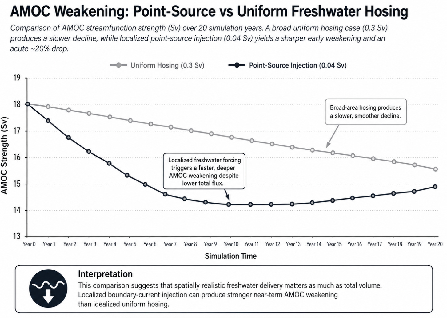
A Sverdrup (Sv) is exactly one million cubic meters of water moving per second (1,000,000 m³/s). It is the standard unit of measurement for volumetric transport in oceanography, designed to quantify the massive circulation of oceanic currents.
To establish the physical scale of this unit, the combined discharge of every river system on Earth draining into the oceans totals approximately 1.2 Sverdrups.
A volume of 0.3 Sv equals 300,000 cubic meters of water per second. This is roughly one-quarter of the entire global river discharge. It significantly exceeds the output of the Amazon River, the largest river on Earth, which discharges at approximately 0.2 Sv.
The structural divergence between these methodologies carries immediate implications for global risk assessment. Utilising uniform averaging embeds an artificial stability into climate forecasts. It effectively masks the acute, localised gargantuan salinity degradation occurring in the Greenland and Labrador currents.
Relying on these diluted models can only lead to a severe structural underestimation of AMOC collapse timelines.
Applying realistic geography fundamentally alters the forecasts. High-resolution models utilising spatially distributed Greenland meltwater inputs averaging 0.04 Sv immediately trigger a 20% weakening of the AMOC at subpolar latitudes. Risk models must integrate local geographic realities to generate accurate outputs. Methodological choices that ignore physical topography guarantee predictive failure.
That sounds technical, but the idea is pretty simple. If the AMOC weakens, it can carry less salty water north. The North Atlantic then becomes fresher. Fresher water is lighter. Lighter water sinks less. That can weaken the AMOC further. Remember, it’s an overturning current, so it circulates from shallow to deep. If the water won’t sink as fast as it did before, it slows down.
Lets step through the modelling layers :
Layer One: Uniform Averaging (The Illusion of Stability)
Standard models apply a uniform averaging methodology.
This approach distributes simulated meltwater evenly across vast ocean grids, treating the North Atlantic as a homogenised catchment area.
The model calculates density shifts by dividing total freshwater volume by the total surface area. This mechanism artificially dilutes the volume, creating a shallow, widespread layer of slightly fresher water. It generates a forecast of a slow, linear deceleration of the AMOC.
Layer Two: Point-Source Hosing (The Mathematical Proxy)
This is a vast improvement on Layer 1. High-resolution models utilise point-source hosing to correct the broad-grid error. This method injects freshwater at specific, localised coastal coordinates. Concentrating the total volume into narrow boundary currents forces the model to process acute density drops.
The structural divergence between Layer One and Layer Two is severe. As shown by the data, point-source injection immediately reduces the AMOC by 20% at subpolar latitudes. Uniform averaging mathematically masks this acute localised degradation.
Layer Three: Physical Reality (The Unmodeled Truth)
Point-source hosing remains a gross estimate. It acts as a static, idealised mathvector.
Physical reality operates through topographically defined mechanisms. Terrestrial and subglacial geology dictate the actual dynamics of meltwater. Ice sheet runoff flows into specific subglacial valleys, pools in massive internal reservoirs, and accelerates through deep, narrow fjords.
These geological funnels discharge high-velocity, seasonal pulses of extreme freshwater concentration directly into the East Greenland and Labrador boundary currents.
Current point-source models inject a steady, localised mathematical stream. Reality delivers concentrated physical bursts that create buoyancy anomalies far exceeding modelled parameters.
To give readers a visual understanding of the run off and the modelling problem, this is a picture of the Greenland coast

The Greenland ice sheetThe coastline, where meltwater is discharged into the ocean, is part of a complex, fjord-indented perimeter estimated to be over 44,000 kilometres (27,000 miles) long. This is if you walked the coast and measured it with a tape measure.
While the entire coastline doesn’t produce equal amounts of meltwater, the ice sheet is surrounded by hundreds of marine-terminating glaciers that deliver meltwater directly into coastal waters.
The true structural risk to the AMOC lies in this third layer, which is too complex for our models to capture.
Risk assessments must evolve past the debate between broad averaging and localised hosing to integrate the physical mechanics of topographical meltwater discharge. Methodological choices that ignore physical topography guarantee predictive failure.
Biology can change ocean heating
The ocean is not just water. It is also biology that impacts climate outcomes.
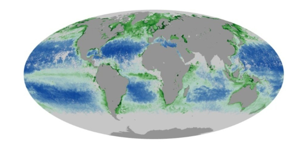
Phytoplankton They are microscopic marine plants. They sit near the base of the ocean food web. They also contain chlorophyll, the green pigment that helps plants and algae absorb sunlight.
Chlorophyll affects how sunlight moves through water.
Where phytoplankton are dense, more sunlight is absorbed near the surface. Where the water becomes clearer, more light can penetrate deeper. Think of it like dark sunglasses vs. light.
Why that’s important: sunlight becomes heat when it is absorbed.
So if ocean biology changes, the ocean’s physical heating pattern can change too.
Changes in chlorophyll can affect where solar energy is absorbed in the water column. Recent modelling work has found that large changes in chlorophyll fields can create temperature biases, including heat accumulation below the deep chlorophyll maximum.
This visual shows how water clarity can change the depth at which sunlight is absorbed. Chlorophyll-rich water absorbs more energy near the surface. Clearer water can allow more sunlight to reach deeper layers. That can affect the ocean’s vertical heat structure.
Think of how the water in your bath feels different at one level or depth than another
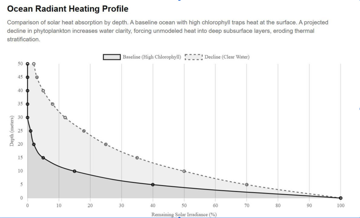
Here, I illustrate a heating profile: chlorophyll-rich vs. clearer waterwith actually data. The baseline is how current AMOC research has modelled it; my decline line is a simulation I ran on probable phytoplankton decline, based on the SST temperatures actually experienced in the region recently.
The modelling problem doesn’t begin only at the ocean boundary. It begins inside the ice sheet. Freshwater hosing experiments usually treat meltwater as an external volume added to the ocean, but real meltwater supply is produced by an ice sheet whose internal state can change unevenly through time.
Dawson et al. show that the basal thermal state of grounded ice can strongly influence future mass loss. Frozen beds resist sliding, thawed beds permit faster flow, and “thawable” beds lie near the pressure-melting point, where a relatively small thermal shift can change the frictional regime beneath the ice. Their Antarctic modelling experiments show that warmer basal conditions can increase mass loss over 100 years, with particular sensitivity in parts of East Antarctica, where frozen-bed patches may help sustain the current ice configuration.
This matters because it changes the meaning of meltwater risk. The freshwater reaching the ocean is not simply a smooth total of surface-melt. It is the output of a thresholded ice-sheet system. Local basal thaw can increase sliding, accelerate outlet glaciers, weaken stabilising ice plugs and open new loci of discharge.
In the George V-Adélie Land region, Dawson et al. describe how local frozen-bed patches may help hold coastal ice plugs in place, and how thawing those patches could contribute to catchment-scale retreat. The general lesson is not limited to Antarctica: ice-sheet discharge can be governed by small, localised, poorly observed control points whose failure changes the behaviour of a much larger system. Think of this as thousands of little ice-made beaver dams (without the beavers)
For AMOC risk, this strengthens the case against treating freshwater hosing as a uniform, slowly changing boundary condition. The ocean doesn’t receive meltwater from an abstract ice sheet. It receives it from a physical ice sheet with basal thermal thresholds, subglacial drainage, topographic funnels, fjords, outlet glaciers, seasonal pulses and possible plug-like controls.
A model that smooths freshwater across a wide grid is therefore simplifying two systems at once: the ice-sheet process that generates the freshwater and the ocean process that receives it. The result can make a thresholded supply chain look like a gradual flux.
My purpose here is to illustrate the model-versus-territory point. One coupled system impacts an adjacent system; more freshwater melt means less plankton, which clears the water, enabling heat to reach much deeper depths.
Sudden aerosol changes can expose hidden warming
Another example is the 2020 shipping fuel rule, known as IMO 2020.
The International Maritime Organisation reduced the allowed sulphur content in most ship fuel from 3.5% to 0.50% starting on 1 January 2020. This was mainly an air-quality and health rule. Sulphur pollution harms human health and contributes to acid rain.
Ships have been releasing these aerosols, initially from coal-fired steam ships, via marine sulphur since the 1830s, when screw propellers were invented, and steam ships took off.
Sulphur dioxide from ships forms tiny airborne particles called aerosols. Aerosols can reflect sunlight, which is called albedo, and brighten some clouds. That means they can have a cooling effect.
Those sulphur particles also form cloud condensation nuclei (CCN), most folk don’t know that clouds are formed when evaporation occurs
So when sulphur pollution was cut, some of that cooling was reduced.
If you remember that phytoplankton we discussed earlier, the ones which we were reducing by increasing the fresh water melting into AMOC, so the heat, in turn, could penetrate more deeply, yet another major source of cloud-condensation nuclei (CCN) is dimethylsulphide, which is produced by planktonic algae in seawater, which oxidises in the atmosphere to form a sulphate aerosol
Because the reflectance (albedo) of clouds (and thus the Earth’s radiation budget) is sensitive to CCN density, biological regulation of the climate is possible through the effects of temperature and sunlight on phytoplankton population and dimethylsulfide production.
Radiative forcing is a measure of how much something changes Earth’s energy balance. Positive forcing means more energy is being retained or absorbed. Negative forcing means more energy is being reflected away.
Several studies estimate that IMO 2020 created a positive radiative forcing, but the size is debated. One study estimated about +0.2 W/m² over the global ocean, with a North Atlantic mean around +0.56 W/m² and regional peaks around +1.4 W/m².
So let’s recap, we lost the sulphur aerosols from ships due to IMO 2020, we lost some more when the freshwater meltwater increased due to freshwater hosing because we killed the phytoplankton, which allowed more heat to get in, which melted faster, which killed phytoplankton
Sudden aerosol changes can alter the amount of sunlight reaching the ocean, especially along shipping lanes. The event shows why abrupt real-world changes shouldn’t be smoothed into harmless-looking long-term averages
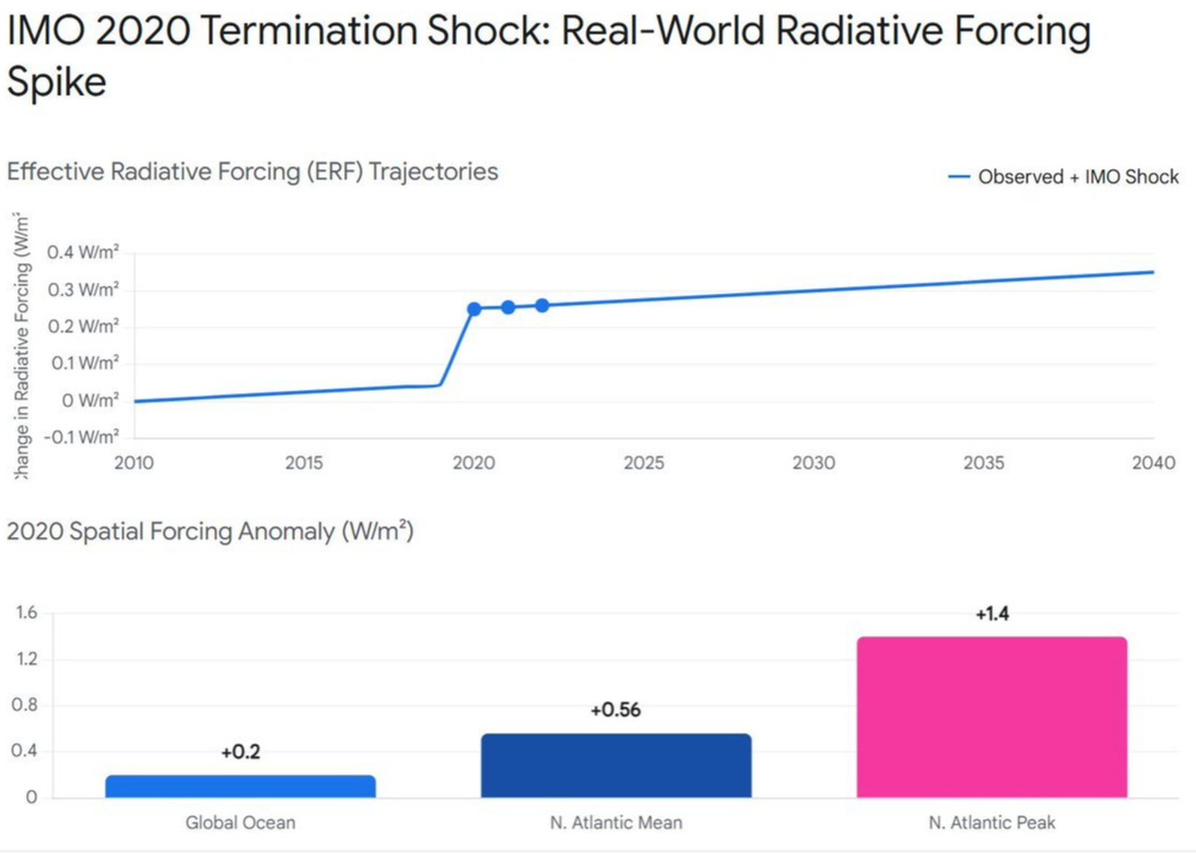
IMO 2020 sharply reduced sulphur pollution from shipping. That improved air quality, but it also reduced some aerosol-related cooling. Estimates of the warming effect differ, but some studies find strong regional forcing over busy shipping regions, especially the North Atlantic.
In fact, this paper argues that the cessation of burning sulphur is responsible for most of the increased heat we are experiencing. This study argues that CERES data show albedo-driven solar absorption explains recent warming and ocean heat, leaving no observed extra greenhouse forcing, implying lower climate sensitivity and overstated climate-model feedbacks overall.
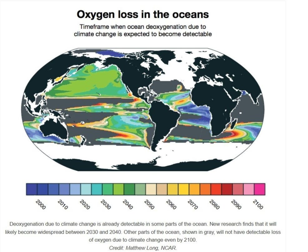
Marine deoxygenation
Marine deoxygenation. This is where surface warming reduces oxygen solubility and strengthens upper-ocean stratification, while freshwater inputs further increase buoyancy contrasts.
This suppresses vertical ventilation and reduces oxygen resupply to subsurface and intermediate waters.
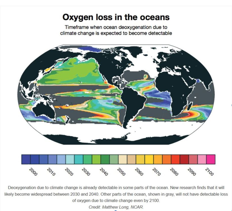
Direct observations indicate that the global ocean oxygen inventory is declining, and models consistently project continued deoxygenation, though with major uncertainties in regional patterns, thermocline trends, temporal variability, and air-sea gas fluxes.
Under low-oxygen conditions, microbial nitrogen cycling shifts toward pathways such as nitrification under oxygen stress, nitrate reduction, and denitrification-linked processes.
These pathways can produce N₂O, especially near oxic-anoxic boundaries where oxygen is low enough to alter microbial metabolism, but physical mixing can still connect dissolved gases to the surface. However, N₂O is not produced and vented automatically.
It can also be consumed by microbes, retained below the mixed layer, diluted, or released later through upwelling and seasonal mixing. That is why the feedback is scientifically plausible but not globally resolved. Marine N₂O hotspots are real, but net atmospheric flux depends on production, consumption, storage, and ventilation.
The drivers are global, the emissions are spatially uneven, and the strength of the feedback remains impossible to model. A PNAS global reconstruction estimated oceanic N₂O emissions at 4.2 ± 1.0 Tg N per year, with 64% from the tropics and 20% from coastal upwelling systems that occupy less than 3% of the ocean area.
That proves the mechanism is hotspot-driven. But because those hotspots are linked to low oxygen, productivity, upwelling, and stratification, global warming can plausibly alter their size, intensity, and atmospheric connections.
Climate change is expanding the global conditions that allow regional nitrous oxide hotspots to form or intensify. Warming reduces oxygen solubility, freshwater inputs strengthen surface stratification, and reduced vertical mixing limits oxygen delivery to deeper waters.
As oxygen declines, microbial communities increasingly rely on nitrogen-based respiration pathways, some of which produce nitrous oxide. Because N₂O has a 100-year global warming potential 273 times that of CO₂, even regionally concentrated increases matter climatically. The logical leap would be to claim that all oceans are now venting N₂O at dangerous rates.
Global deoxygenation is weakening the ocean’s stabilising role, while specific low-oxygen and upwelling regions may become stronger sources of high-impact greenhouse gases. This makes marine deoxygenation a plausible climate feedback, but one whose global strength remains uncertain.
The striking feature of the global maps is not any single layer. It is the overlap. Historic shipping-sulphur corridors trace the fixed industrial arteries of the ocean. Phytoplankton maps show where the surface ocean is biologically active enough to shape carbon cycling, cloud chemistry, light absorption and food-web stability. Deoxygenation maps show where warming and stratification are expected to make oxygen loss detectable first. When these layers are placed beside one another, the coincidence is not random-looking. It is especially suggestive in the North Atlantic, where major shipping corridors intersect with phytoplankton-rich waters, aerosol-sensitive cloud regimes, Greenland freshwater pathways and the broader AMOC system. That does not prove a causal chain by itself. It defines the test. If the same ocean surface is being aerosol-altered from above, chemically loaded from ships and runoff, biologically stressed through phytoplankton and DMS pathways, and physically freshened by meltwater, then the relevant risk is not one mechanism in isolation. It is industrial surface-ocean coupling: a no-analogue forcing layer sitting directly on top of circulation machinery.
The Moving Pole: Ice, Water, Ocean Circulation and Earth’s Spin
The Earth is not a fixed ball spinning cleanly through space. Its rotation axis moves. The pole wanders across the surface in loops, spirals and drifts. That movement is measurable. Think of it as a wobbly top you had as a child .
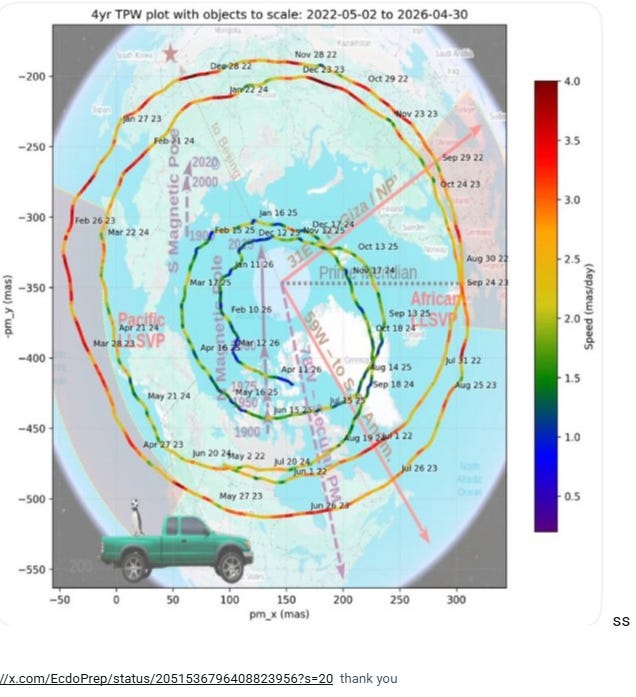
The polar excursion map shows this directly.
The line traces the position of Earth’s rotational pole across time. The loops reflect seasonal and longer-period motions, including the Chandler wobble. The colours show speed. The important point is simple: Earth’s axis is not locked. It responds to the planet’s mass distribution


thank you
Modern polar motion is plotted as a moving path of Earth’s rotational pole. The spiral shows the pole’s changing position through time. Wider loops indicate stronger wobble; tighter loops indicate reduced amplitude. The colour scale marks velocity. The map is not showing the magnetic pole. It is showing the movement of Earth’s rotation axis relative to the crust.
Move enough mass, and the planet rebalances. If you’ve done pottery, the physics isn’t much different. Melt the ice in Greenland, and it redistributes add to Earth’s wobble
Ice melts. Groundwater is pumped. Soil dries. Oceans gain water. Sea level redistributes unevenly. The solid Earth rebounds after ice is removed. All of this changes Earth’s inertia. The spin axis adjusts.
Polar motion is a visible signal of mass redistribution across the Earth system. AMOC reorganisation is part of that system because it shifts heat, freshwater, density, regional sea level and ice stability. The pole responds to the mass geometry produced by the coupled ice-ocean-land-water system.
NASA/JPL states that climate-related redistribution of ice and water has nudged Earth’s spin axis by about 10 metres over the past 120 years and is also lengthening Earth’s day. The drivers include melting ice sheets, melting glaciers, groundwater loss and rising seas.
Groundwater alone has already left a measurable fingerprint. A 2023 Geophysical Research Letters study found that groundwater depletion shifted Earth’s rotational pole about 80 centimetres east between 1993 and 2010. So, pumping all the groundwater we’ve pumped, we’ve also changed Earth’s spin . When you start to see all these couple of earth systems, you start to realise the specialist way we are studying these systems doesn’t serve our ability to detect risk.
The Chandler wobble adds another clue. It is a natural wobble in Earth’s rotation with a period of roughly 14 months. A 2025 Journal of Geodesy study found that recent changes in the Chandler wobble are better explained when hydrological, cryospheric and sea-level mass changes are included.
https://link.springer.com/article/10.1007/s00190-025-02021-w?utm_source=chatgpt.com
This means the modern pole is already carrying a water-and-ice signal.
The first chart isolates the Chandler wobble by stripping away the slow background movement, so what you see are clean, repeating loops around a fixed point. That’s useful if you only care about the wobble itself. But the Earth doesn’t behave like that in reality. The axis is not just wobbling in place, it is also slowly migrating because mass is being redistributed across the planet. When we put the trend back in, as in the second chart, those same loops no longer sit still; they move across the surface, revealing the underlying drift. A simple way to picture it: a spinning top wobbles naturally, but if you stick a bit of chewing gum on one side, it not only wobbles, it starts to shift position as it spins. The first chart shows the wobble after removing the gum’s effect. The second shows the actual system, where wobble and drift happen together.
This final chart strips the idea down to its simplest form.
Instead of comparing filtered and unfiltered signals, it shows the pole’s actual path through time as a sequence of migrating loops.
The key observation is that the loops do not remain centred in one place. Their centre slowly shifts across the graph, meaning the Earth’s axis is not merely wobbling, it is wandering.
The earlier Chandler wobble chart isolated the oscillation by mathematically removing the long-term movement. The wobble-and-drift chart then restored that movement, revealing the hidden migration beneath. This chart brings both ideas together in a single image: the wobble is the repeating loop, while the changing positions of the loops reveal the underlying drift caused by the redistribution of mass across the Earth system.
AMOC belongs inside this same machinery; it’s all coupled together, we live on a top that’s spinning, and our civilisation is adding or removing chewing gum, and as a result, the top is wobbling
The AMOC is the Atlantic Meridional Overturning Circulation. It moves warm surface water northward and returns colder, denser water southward at depth. It depends on temperature, salinity and density. Add freshwater to the North Atlantic, especially from Greenland melt, and surface water becomes less dense. That can interfere with deep-water formation.
But the key point is this:
AMOC reorganisation and polar motion are linked through mass redistribution.
AMOC change shifts heat. Heat shifts ice stability. Freshwater shifts density. Density shifts ocean structure. Ocean structure shifts the regional sea level. Ice loss shifts mass from land to ocean. The pole responds to that whole geometry.
The ENSO measurement problem
The same issue appears in near-term climate forecasting.
ENSO means El Niño-Southern Oscillation. It is a natural climate pattern in the tropical Pacific that can shift weather worldwide.
El Niño is the warmer phase.
La Niña is the cooler phase.
The Niño-3.4 region is a specific part of the tropical Pacific that scientists use to track ENSO.
NOAA now uses the Relative Oceanic Niño Index (RONI) to assess ENSO strength probabilities. RONI starts with temperature anomalies in the Niño-3.4 region, subtracts the average tropical sea-surface temperature anomaly, and then adjusts the result so that its variability matches that of the older Niño-3.4 index. NOAA says this helps track El Niño and La Niña more reliably in a warming tropical ocean.
A relative index is useful for identifying the contrast between the Niño-3.4 region and the wider tropics. This Index is the one you look at when trying to assess El Niño probability and strength
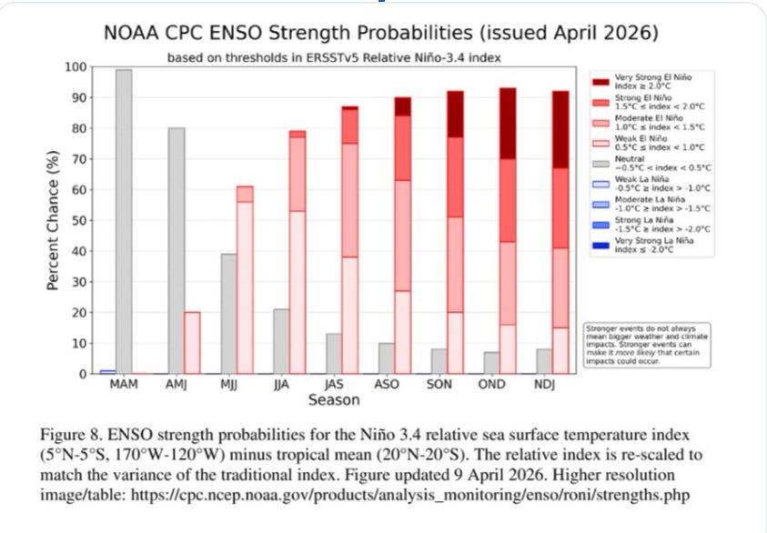
The relative index is computed by subtracting the 30-year tropical mean. This calculation effectively maps geographic weather displacement. It simultaneously deletes the absolute heat from the risk ledger, obscuring the physical payload entering the biosphere.
But again, it does not tell the whole risk story. It’s like trying to pass off a chapter of a textbook as a whole textbook
Crops, reefs, evaporation, workers, power grids, and supply chains respond to absolute heat stress. They don’t care whether the heat is counted as background warming or as an ENSO anomaly.
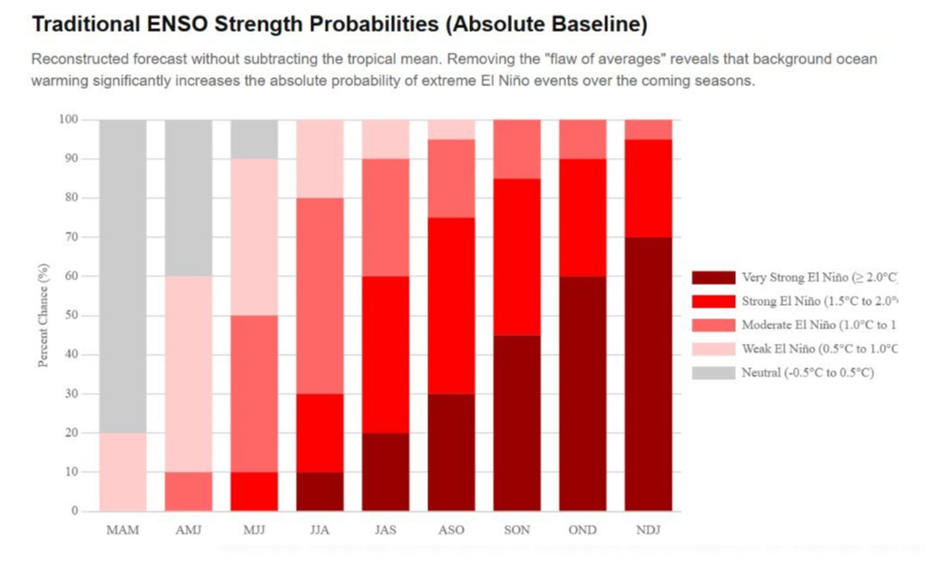
So let’s redo the chart anew without the 30 Year average dilution. The new chart escalates the risk of a very strong El Niño significantly
The question is, what risk are we trying to measure?
If we are forecasting shifts in weather patterns, a relative index can certainly be useful. (The First Chart)
If we are assessing physical heat stress on ecosystems, agriculture, and infrastructure, absolute heat also matters. (The 2nd Chart)
NOAA’s official ENSO strength probabilities (1st Chart) use the Relative Oceanic Niño Index. This is designed to track El Niño and La Niña by contrasting the Niño-3.4 region with the wider tropics. NOAA’s April 2026 strength table shows probabilities across overlapping three-month seasons and classifies events by relative Niño-3.4 thresholds.
This comparison (2nd Chart ) uses an absolute-baseline view to show total thermal stress rather than only the relative ENSO pattern. This is a way better risk lens, not as an official NOAA forecast. But ideally, we should have both, yet only the former is considered a risk model.
I hope the message you’re getting is that these systems are really complex, coupled and dynamic; they are very hard to model, and each model can justify different approaches to each variable for different reasons.
The Darkening Planet: Separating Physics from Panic
To grasp the systemic risk, we have to look beyond localised ocean currents and shipping regulations to the absolute thermodynamic ceiling of the planet: Earth’s albedo.
In layman’s terms, albedo is planetary reflectivity. It is a measure of how much incoming solar energy is reflected by white surfaces, such as sea ice, snow, and dense clouds, and is returned to space. It acts as Earth’s primary thermal shield.
When ice melts into dark ocean water, or when atmospheric heating thins out marine cloud layers, the planet loses its mirror. A darker Earth absorbs more heat, which melts more ice, which darkens the Earth further. It is the ultimate, irreversible physical feedback loop.
This chart is a mechanical observation of energy already accumulated.
This massive injection of unmodelled heat is the exact physical force currently eroding the deep-water thermal stratification we discussed earlier.
Remember, from the less sulphur from the phytoplakon and marine fuel, the fewer sulphur particles to form clouds, the more heat in, the more fresh water melts in, the less phytoplankton, the deeper the extrasolar energy penetrates
It is the energy powering the sudden atmospheric shifts, destabilising the AMOC. It is the exact thermal pressure driving global evaporation rates past the breaking point of our agricultural supply chains.
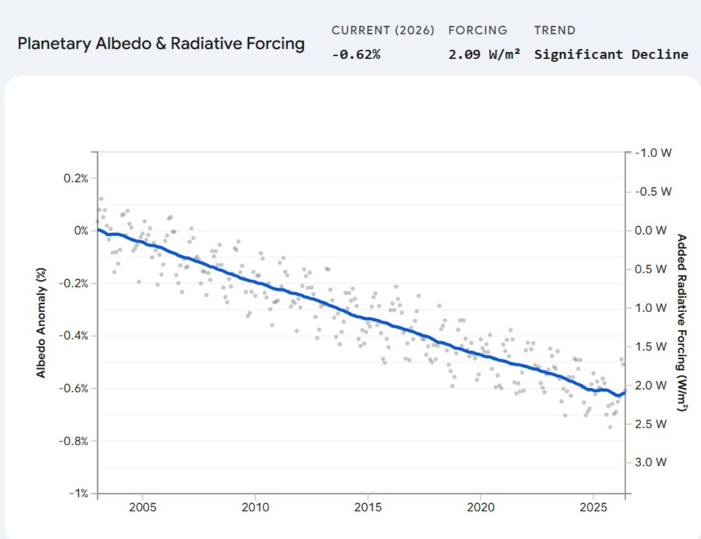
Earth’s albedo is falling, meaning the planet is reflecting less sunlight back into space and absorbing more of it instead. The current decline, about 0.62 percentage points, corresponds to roughly 2.09 W/m² of additional solar energy being absorbed globally. This metric translates to the equivalent thermal energy of hundreds of thousands of atomic detonations occurring continuously across the Earth’s surface. In practical terms, Earth’s climate system is now taking in significantly more energy than it used to, and unless that reflectivity recovers, the planet must warm until it can radiate that extra energy back to space.
ScenarioMIP-CMIP7 and the Smoothing of Tail Risk
This ScenarioMIP-CMIP7 paper is useful, serious, and incomplete.
It is useful because it provides the climate-model community with a coherent set of seven scenarios, pushes more simulations into CO₂ emissions-driven mode, and adds long extensions to 2150 and 2500 to study overshoot, stabilisation, and reversibility.
A foundational glossary defines the assessment architecture: Integrated Assessment Models (IAMs) operate as economic simulators that estimate future emissions, while Earth System Models (ESMs) operate as physical climate simulators that process those emissions into warming and weather patterns.
It is incomplete because those same design choices are built for coordination and tractability, not for exposing the ugliest edge of the risk distribution. The core framework is bounded by “plausible” scenarios, not by a full tail-risk envelope. It narrows the upper end relative to CMIP6, uses marker pathways to stand in for wider IAM uncertainty, assumes away climate damages inside the scenario construction, and presents headline outcomes with central summaries that do not describe the dangerous tails.
That matters because the Intergovernmental Panel on Climate Change has already said that low-likelihood, high-impact outcomes such as abrupt ocean circulation changes, compound extremes, and warming above the assessed very likely range cannot be ruled out and should be included in risk assessment.
AR6 is equally clear that multi-model means and ensemble spreads are not sufficient where models produce different or even opposite outcomes, and that high-warming storylines can produce regional changes far larger than the multi-model mean. ScenarioMIP-CMIP7 partly recognises that problem, but mostly pushes it to future work.
ScenarioMIP-CMIP7 does contemplate some high-end risk, but it under-represents upper-tail climate risk in the places that matter: abrupt circulation change, aerosol unmasking, marine biological feedbacks, compound correlated tails, CDR failure, and the possibility that climate damages feed back into the socio-economic pathways that generated the scenarios in the first place. It should be treated as a standardised experiment suite, not as a complete map of climate risk.
What the paper explicitly does, what it postpones, and what it misses
A. What the paper explicitly does. The protocol proposes seven core scenarios for 2025–2100, spanning High through Very Low, plus overshoot and negative-emissions variants. It prioritises CO₂ emissions-driven runs wherever possible, provides concentration pathways for models that cannot run that way, and asks for long extensions to 2150 for all scenarios and to 2500 for at least two priority extensions, preferably High and Very Low.
It also recommends at least five ensemble members per scenario to sample internal variability, especially near the low end, where separating scenarios is harder. These are sensible design choices for a coordinated intercomparison.
B. What the paper acknowledges but pushes outside the core framework. The paper says plainly that not all important questions fit inside ScenarioMIP. It recommends wider sets of IAM scenarios, including idealised or counterfactual paths above or below the plausible range. It recommends alternative IAM implementations of the same qualitative scenarios.
It recommends scenarios that include climate impacts, and it explicitly states that adaptation-mitigation interactions are not currently considered in how information moves across communities. It also says that relative likelihoods beyond the crude judgment of “plausible or not” should be characterised in future work, and that atmospheric chemistry uncertainty would be better represented by running emissions through multiple chemistry models rather than a single one. In other words, the paper knows the core suite is not enough.
C. What the paper misses. There is no dedicated treatment of AMOC, the Atlantic overturning collapse, or freshwater hosing, despite generic references to tipping points and irreversibility.
Searches also return no explicit discussion of phytoplankton, chlorophyll, DMS, deoxygenisation, or NPP, even though the same paper devotes long sections to CDR workflow and land-based mitigation. That is enough to show the frame of concern: the protocol is explicit about mitigation architecture and carbon accounting, but it is thin on abrupt ocean circulation risk and ocean-biosphere feedbacks.
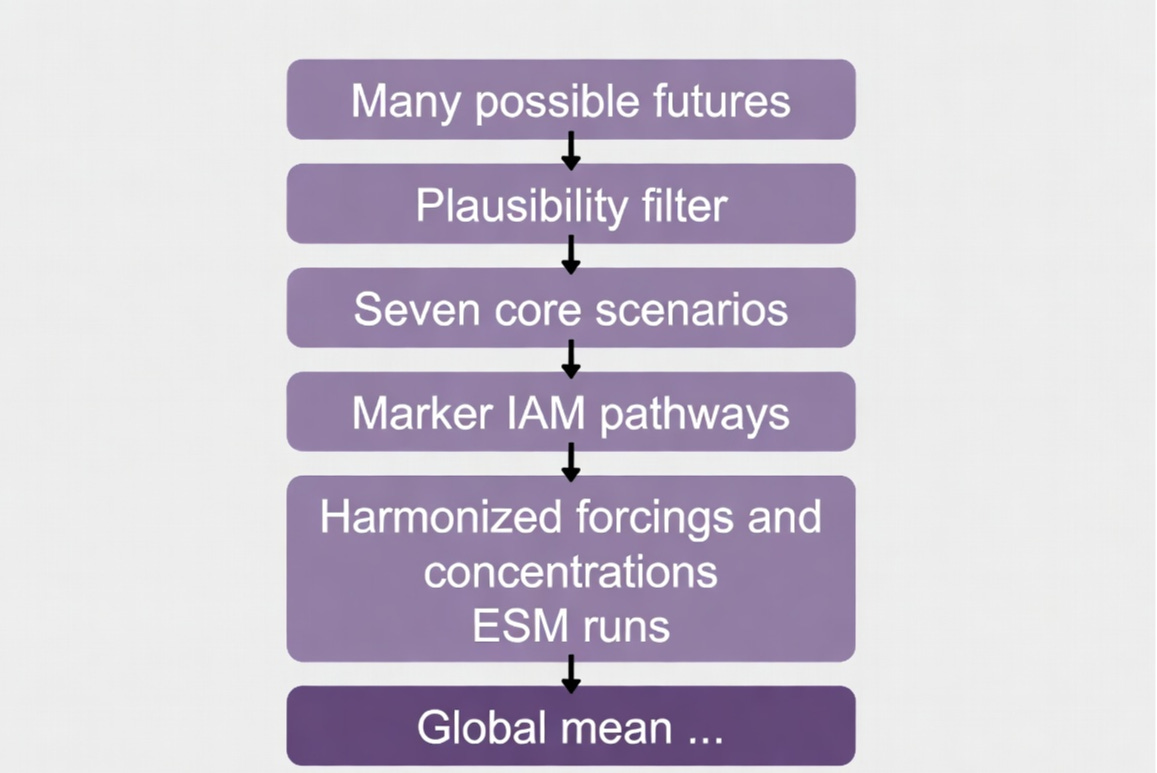
Figure 1 is a schematic, not a reproduced figure from the paper. It shows the compression chain that the ScenarioMIP protocol itself describes: plausibility filtering, marker selection, harmonisation, chemistry simplification, and summary by central outcomes rather than by tails.
Where the framework compresses tail risk
High-tail risk. The framework underplays tail risk by construction. The paper defines its scenario set as a broad yet plausible range, states that plausibility is subjective, holds plausibility judgments conditional on the assumption that there are no climate impacts within the scenarios, and acknowledges that there may be futures outside the ScenarioMIP range.
It further says that likelihood judgments are currently limited to whether scenarios are plausible, with only a loose suggestion that the High and Very Low scenarios may be less likely than the middle cases.
The implication: if the protocol starts from bounded plausibility rather than from stress-testing what could break badly, it will compress risk before modelling even starts.
Global averages and central summaries. The framework relies too heavily on central tendency. The paper’s own summary figure shows the 33–67 percentile range for temperature outcomes around the marker scenarios. For concentration-driven runs, it recommends the median concentration pathway from carbon-cycle emulators.
And it openly notes that a forcing difference large enough to separate global mean temperature by about 0.25–0.3°C may be needed to generate distinguishable outcomes across scenarios, while admitting that the current set may be separated by somewhat less.
The implication is that subtle but policy-relevant differences could be lost in noise, especially for regional extremes, while threshold outcomes get averaged into something that no model member actually produces.
Why the mean is a bad risk lens. AR6 WG1 says this directly: the multi-model mean and ensemble spread are not sufficient when different models produce substantially different, or even opposite, regional changes. It also says that low-likelihood, high-impact outcomes cannot be ruled out, that compound extremes become more frequent with warming, and that high-warming storylines can show far larger regional temperature, drying, and wetting changes than the multi-model mean.
The policy implication is brutal: if planning relies on the “threshold crossed” and “threshold not crossed” dichotomy, it will systematically under-plan for the state that actually arrives.
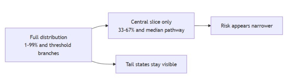
Figure 2 is a schematic of the central problem. ScenarioMIP does not hide uncertainty, but its default presentation emphasises the middle of the distribution when the relevant loss functions often sit in the tails.
Regional risk. Claim: the protocol leans too hard on global-forcing equivalence. The paper says ESM results from one ScenarioMIP pathway can often be used with alternative socio-economic pathways or mitigation strategies as long as global forcing is similar, then immediately admits that existing evidence is limited and that regional forcing differences from short-lived climate forcers or land use may matter.
AR6 WG1 says: regional climate change emerges from the interaction of external forcings, internal variability, and non-linear feedbacks, with land-use and aerosol forcing playing important roles in extremes and even in the sign of some regional precipitation changes.
The implication is that “same global forcing” is not the same as “same
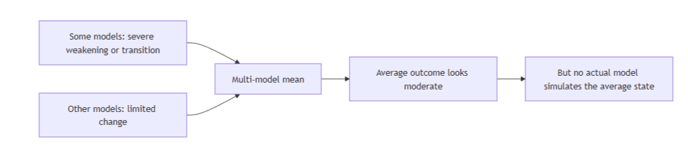
Figure 3 shows why threshold systems punish averaging. For AMOC, low-cloud states, or ecosystem regime shifts, the mean of incompatible model states is often not itself a physically realistic state.
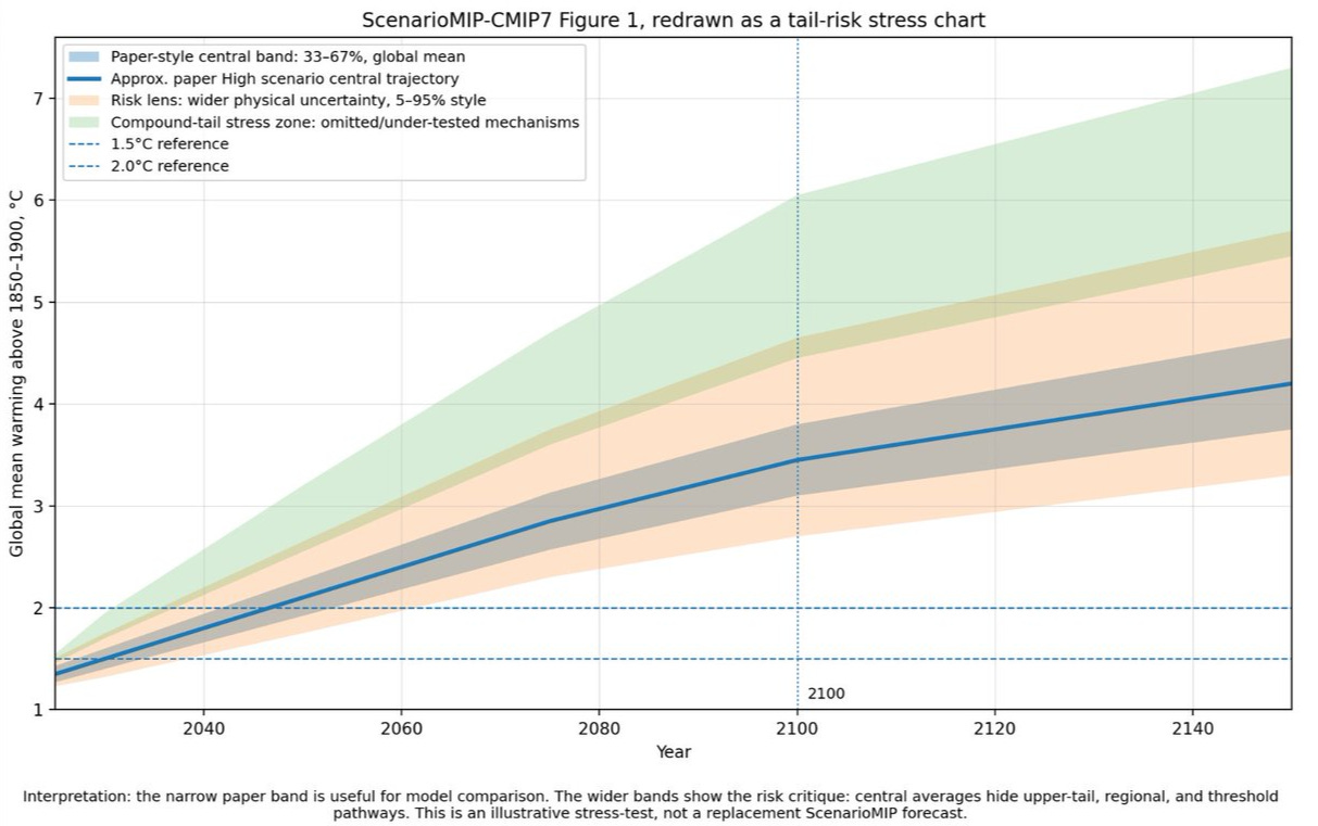
So I re-did the chart in the paper (blue line) and adjusted it for the compounded coupled risks, and you see the risk becoming much more severe
AMOC, aerosols, and the marine biosphere
AMOC. The framework does not explicitly test AMOC weakening or shutdown. The ScenarioMIP paper contains no AMOC-specific scenario, no freshwater-hosing experiment, no Greenland-melt sensitivity branch, and no AMOC diagnostics embedded in the core protocol.
The paper reaches 2500 for selected extensions and mentions tipping points in general, but generic long runs are not the same as deliberate AMOC stress tests.
Ditlevsen and Ditlevsen estimated a possible mid-century collapse under continued forcing; a 2025 Nature study found AMOC resilient to extreme greenhouse-gas and freshwater forcing across 34 models; and a 2025 long-run analysis found that northern Atlantic overturning shutdown after 2100 emerges in some CMIP6 futures, while also noting that abrupt collapse in the strict sense is usually seen only in idealised hosing experiments.
The right implication is not that the shutdown is certain. It is that the uncertainty is now too consequential to leave outside the core protocol.
Aerosols and abrupt unmasking. The framework under-tests the uncertainty in aerosol forcing and abrupt aerosol unmasking. The paper says non-CO₂ gases and air pollutants will mainly be imposed through atmospheric concentrations, with a single atmospheric chemistry model providing concentration fields, and it says a fuller uncertainty treatment would require “additional chemistry models”. Evidenced by some of the forcings I have mentioned in the paper, it’s not just chemistry we should be examining, it’s the physics of all the coupled systems.
The International Maritime Organisation sulphur rule Cut the global sulphur cap in marine fuel from 3.5% to 0.50% from 1 January 2020, with the IMO forecasting a 77% drop in overall ship SOx emissions. Peer-reviewed estimates of the associated radiative forcing span roughly 0.06–0.09 W m⁻² in a multi-model estimate, about +0.074 ± 0.005 W m⁻² in a machine-learning observational estimate, about +0.12 to +0.13 W m⁻² in recent model studies, and +0.139 ± 0.019 W m⁻² in one Earth’s Future estimate. A 2025 ACP study then argued that while the forcing is real, its global-mean surface-temperature effect remains hard to detect above internal variability so far.
That aerosol unmasking is real and uncertain; mixed on how much of the recent global mean temperature jump it explains. The implication: a risk framework should branch this uncertainty explicitly rather than compress it into a single chemistry realisation.
Regional aerosol effects. The protocol treats a strongly regional forcing problem too globally. Shipping aerosols act on clean marine-cloud regimes, not on the planet evenly.
A 2025 Nature Communications study found marine cloud reflectivity over the combined North Atlantic and Northeast Pacific fell by 2.8 ± 1.2% per decade from 2003 to 2022, with reductions in sulphur dioxide and related aerosol precursors explaining about 69% of the decline through aerosol-cloud interactions.
The same study found that the majority of Earth system models simulated weaker cloud-reflectivity and SST trends than observed. Evidence strength: strong. The implication is that tail-risk work should not hide shipping-lane and basin-scale forcing behind global means.
Marine biology. The framework underplays marine biological risk. The protocol contains no explicit treatment of phytoplankton, chlorophyll, DMS, or NPP, despite asking long-run questions about reversibility and irreversible change. That omission matters because the marine biosphere is not just a downstream victim of warming. It is part of the climate system.
The IPCC ocean assessment found that upper-ocean nutrients and net primary productivity are projected to decline under high emissions, with global NPP very likely down by 4–11% by late century under high forcing but with low confidence because observations remain limited.
A 2025 Communications Earth & Environment study went further and found that future NPP decline is more likely than previously predicted, and that even the best CMIP6 models still underestimate the sensitivity of NPP decline to ocean warming.
The implication is that a long-horizon Earth-system protocol should not treat ocean biology as an optional detail.
DMS and chlorophyll feedbacks. The feedback is too uncertain and too relevant to ignore. DMS is the largest natural sulphur source to the atmosphere and a source of cloud condensation nuclei, but its emission estimates remain highly uncertain. A 2024 Biogeosciences study says exactly that. A 2024 npj Climate and Atmospheric Science study projects lower future sea-surface DMS and related aerosol radiative forcing than CMIP6 ESMs suggest, with sea-surface DMS down about 16.1% and flux down about 18% by 2099 under SSP5-8.5 in its adjusted estimate.
In this study Marine heatwaves are shaping the vertical structure of phytoplankton in the global ocean , promoting deep chlorophyll maxima and reshaping the structure of subsurface chlorophyll.
The implication is that the coupling among biology, radiative forcing, stratification, and marine heatwaves is robust enough to warrant explicit stress tests. Not because it’s proven, but commonsense evidence demands, particularly because the couple evidence is starting to add up to a very high risk climate future
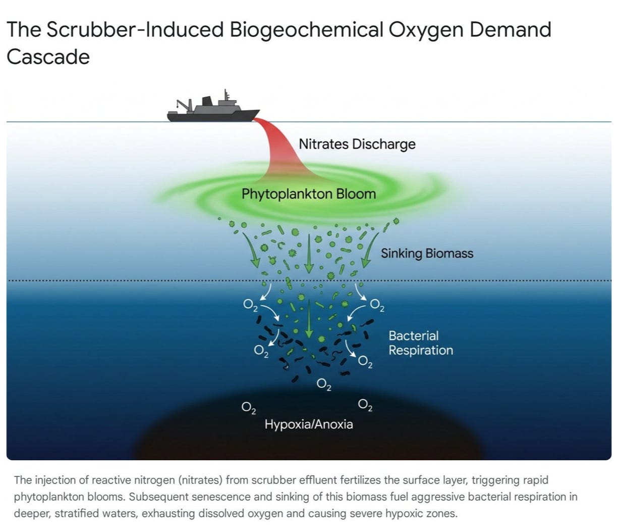
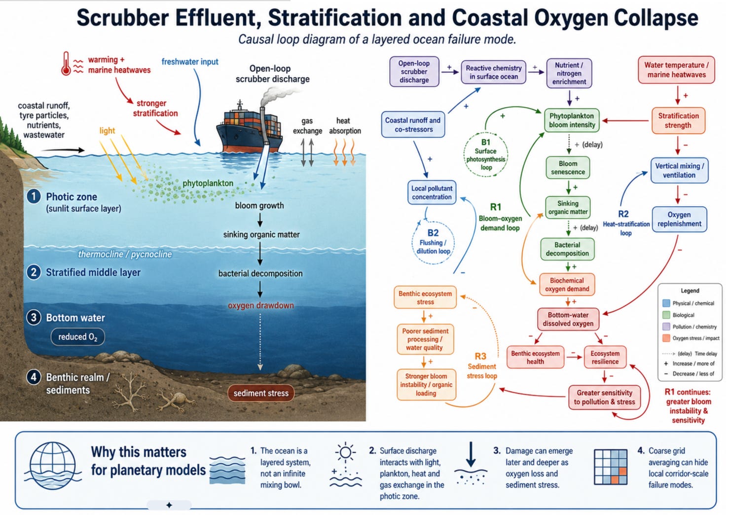
Openloop Scrubber Effluent, Phytoplankton and Deoxygenation
The Industrial Deoxygenation Vector: Methodological Failures in Climate Modelling and the Impact of Maritime Point-Source Emissions
The integrity of global Earth System Models relies entirely on the parameterisation of physical and chemical fluxes. Oceanographic and climate modelling exhibits a persistent structural vulnerability: the translation of highly concentrated, mobile point-source phenomena into grid-scale averages. The ongoing debate surrounding Atlantic Meridional Overturning Circulation (AMOC) “freshwater hosing” experiments exposes this failure. Traditional simulations evaluate ice-sheet deterioration by applying a parameterised “uniform freshwater flux,” smearing meltwater evenly across vast, coarse-resolution oceanic grids.
Uniform hosing mathematically misrepresents heterogeneous melting patterns. Physical freshwater forcing arrives via dynamic icebergs—highly mobile, localised point sources of extreme latent heat extraction and low-salinity water injection. Three-dimensional dynamic iceberg models track these icebergs along specific, narrow trajectories, including the North Atlantic “iceberg alleys” and the Southern Ocean’s Weddell Gyre. This point-source extraction of heat and injection of freshwater severely stratifies near-surface waters, inhibits vertical heat redistribution, and induces extreme, localized surface salinity biases. These anomalies propagate into critical deep-water masses like Antarctic Bottom Water. Uniform grid averaging dilutes these density anomalies, mathematically erasing the localised disruptions that arrest deep-water formation and trigger delayed AMOC equilibrium responses.
The heuristic dilution of localised, high-intensity flux into a grid-average currently plagues the environmental assessment of commercial maritime operations. The global shipping industry operates as a continuous, massive point-source injector of thermal, chemical, and biological disruption. The widespread deployment of Exhaust Gas Cleaning Systems (EGCS), or marine scrubbers, introduces billions of tons of toxic, acidified, and nutrient-dense effluent directly into the marine surface layer. Global biogeochemical models evaluate the impact of these scrubber emissions on ocean acidification and deoxygenation by replicating the AMOC hosing error. They apply the chemical inputs as a uniform flux spread evenly across oceanic regions. This structural error erases the extreme, sub-grid scale reality of shipping corridors. It validates the premise of rapid oceanic dilution while missing the severe, localized biogeochemical collapse triggered along high-density transit routes.
The Geography of Risk: Early-Onset Hypoxia in High-Traffic Corridors
The physical manifestation of this modelling failure is evident in the highly stratified, heavily trafficked maritime corridors of the global ocean. Think of these boundaries as impenetrable physical walls formed by temperature and salt density that lock toxic effluent in the surface layer
Anthropogenic climate forcing drives macro-trend deoxygenation; the point-source injection of reactive industrial effluent operates as a potent accelerant, compressing the timeline to acute hypoxia in specific geographic areas
The continuous discharge of scrubber washwater alters the chemical baseline of receiving waters. This environment shifts toward early-onset deoxygenation ahead of baseline climate predictions. The most severe impacts localise heavily along the primary arterial routes of global trade, particularly within the North Pacific transit routes, the dense shipping networks of the North Atlantic, and critical maritime chokepoints where physical geography limits lateral dispersion and tidal flushing.
Hydrodynamics amplify the disruption caused by point sources within these specific corridors. Estuarine environments, coastal shelf zones, and fjords trap the injected effluent within the photic zone due to vertical stability and long water-mass retention times. A grid-averaged calculation assumes infinite lateral diffusion.
The physical reality relies on density-driven stratification. Thermoclines and haloclines act as impenetrable physical walls formed by temperature and salinity differences, locking toxic effluent in the surface layer and preventing dilution of the scrubber plume.
The integration of exhaust gas cleaning systems into the global maritime fleet establishes a vector for the direct transfer of severe chemical pollutants into the open water column. The physical, chemical, and biological evidence demonstrates that marine scrubbers engineer intense, sub-grid-scale biogeochemical disruptions that threaten both the open-water column and ocean-floor ecosystems along critical maritime transit routes.
Spatial Correlation: The Intersection of Shipping Lanes and Artificial Biological Activity
The causal mechanism linking maritime transit to localised deoxygenation is revealed by the spatial correlation between industrial traffic patterns and surface biological anomalies.
Bulk carrier vessels constitute approximately 22% of the global merchant fleet and serve as primary adopters of scrubber technology. They continually combust high-sulphur residual heavy fuel oil along highly defined, repetitive routes, creating a continuous, linear point-source injection vector across the pelagic ocean.
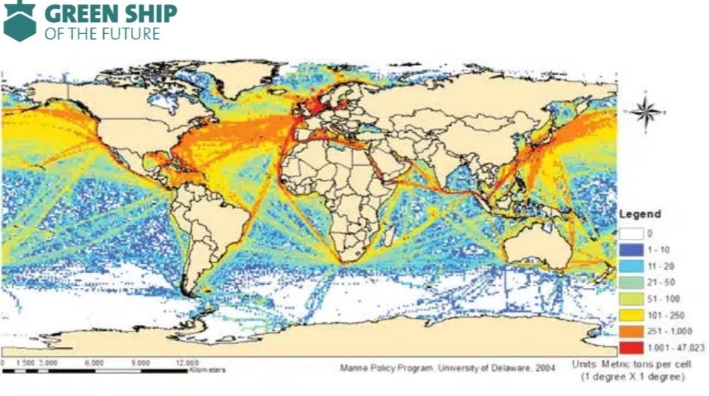
Overlaying high-resolution mapping of global shipping lane density with global phytoplankton distribution reveals a striking spatial correlation. Extreme maritime traffic coordinates perfectly match zones exhibiting persistent, early-onset deoxygenation and artificial biological hyperactivity.
The chemical composition of the scrubber effluent acts as a continuous, fertilisation strip. Anomalous chlorophyll a concentrations trace precisely along these transit corridors.
Coastal and marginal seas experience localised blooms triggered by the influx of anthropogenic nutrients. This spatial signature proves maritime emissions operate at a sub-grid scale, initiating biological feedback loops along narrow geographic bands that broad-grid climate models systematically miss.
The striking feature of the three global maps is not any single layer. It is the overlap of these layers and the implications of those overlaps. Historic shipping-sulphur corridors trace the fixed industrial arteries of the ocean.
Phytoplankton maps show where the surface ocean is biologically active enough to shape carbon cycling, cloud chemistry, light absorption and food-web stability. Deoxygenation maps show where warming and stratification are expected to first make oxygen loss detectable.
When these layers are placed side by side, the coincidence isn’t random-looking. It is suggestive in the North Atlantic, where major shipping corridors intersect with phytoplankton-rich waters, aerosol-sensitive cloud regimes, Greenland freshwater pathways and the broader AMOC system.
If the same ocean surface is being aerosol-altered from above, chemically loaded from ships and runoff, biologically stressed through phytoplankton and DMS pathways, and physically freshened by meltwater, then the relevant risk is not one mechanism in isolation. It is industrial surface-ocean coupling: a no-analogue forcing layer sitting directly on top of circulation machinery
Engineering Architectures and the Physicochemical Transformation of the Water Column
The mechanics driving this spatial correlation are rooted in the engineering architectures of exhaust gas cleaning systems and in the severe physicochemical transformations they inflict upon the ambient water column.
Scrubbers force the absorption of gaseous sulphur oxides (SOx) and nitrogen oxides (NOx) into a liquid medium, shifting pollution from atmospheric emission to aqueous discharge via closed-loop and open-loop designs.
Closed-loop systems operate in estuarine ports and zero-discharge zones, utilising a finite, recirculating freshwater volume.
The system requires continuous injection of alkaline reagents, primarily sodium hydroxide or magnesium hydroxide, to neutralise the severe acidity generated by the dissolution of sulphur. Flocculants bind suspended particles into sludge, which is then separated via multicycles for shoreside disposal. The system discharges a continuous “bleed-off” of highly concentrated, treated washwater to prevent thermal overload and salt precipitation.
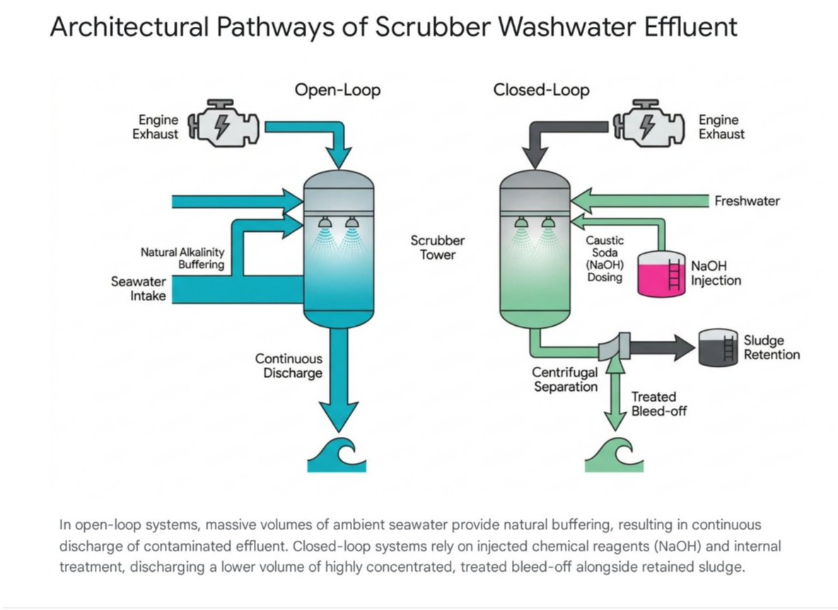
Open-loop systems comprise over 81% of global installations and utilise no internal chemical dosing. They rely entirely on the natural alkalinity of massive volumes of ambient intake seawater to neutralise exhaust acids. Exhaust gases are sprayed with seawater, ionising sulphur dioxide into highly reactive sulphites. The vessel discharges the resulting washwater continuously back into the sea in immense volumes.
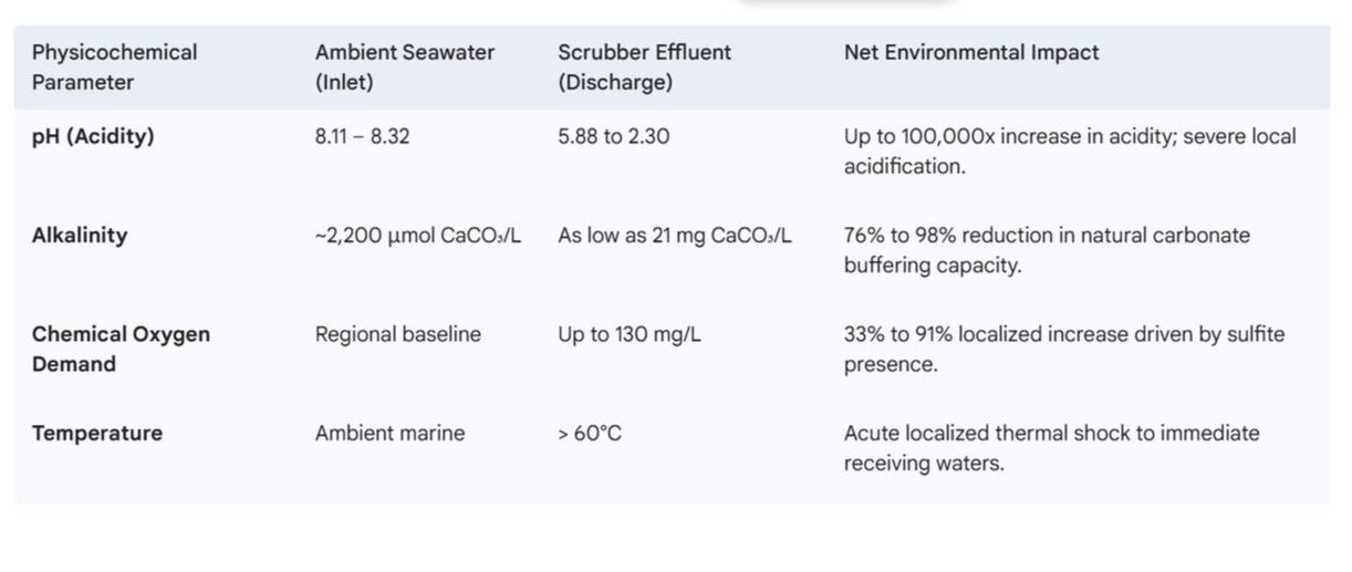
The physicochemical transit through an open-loop scrubber results in a radically altered effluent that inflicts acute chemical trauma on the immediate receiving waters.
Heavy fuel oil combustion byproducts transferred into the washwater include highly recalcitrant polycyclic aromatic hydrocarbons (PAHs) and trace heavy metals such as vanadium, nickel, and lead.
harge at least 10 gigatonnes of washwater each year, with about 80% released within 200 nautical miles of shore, meaning the pollution is concentrated in the same coastal and upwelling zones where oxygen stress is already more likely.
A rough mass-balance estimate suggests open-loop scrubbers may transfer around 0.7-1.3 million tonnes of sulphur per year into the ocean, mostly as sulphate/bisulphite chemistry, depending on fuel sulphur content and scrubber operation.
Heavy-metal loading is smaller but still significant: a Pacific Canada assessment found 88.3 million tonnes of scrubber washwater in 2022 contained nearly 26 tonnes of metals; scaled globally to 10 gigatonnes of washwater, that implies an order-of-magnitude estimate of roughly 3,000 tonnes of heavy metals per year.
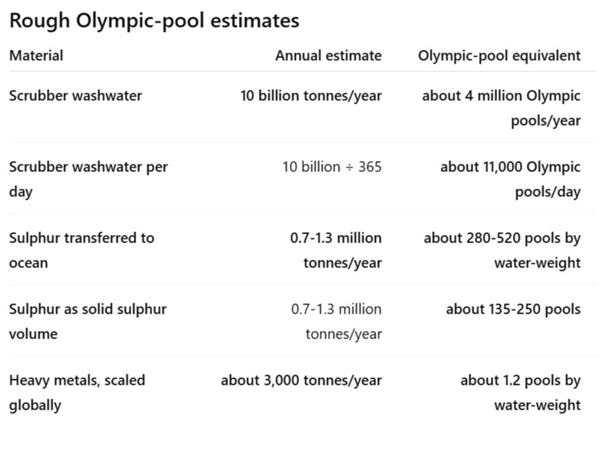
Around 3,000 tonnes per year may sound small beside billions of tonnes of scrubber washwater, but that comparison misses the point. Metals such as vanadium, nickel, copper, lead, cadmium, and mercury can affect marine organisms at very low concentrations, persist in sediments, and bioaccumulate through food webs.
A rough scale illustration shows the issue: 3,000 tonnes is equal to 3 quadrillion micrograms, meaning that even against a simple 1 µg/L benchmark, it would take roughly 3 quadrillion litres of water, or about 1.2 billion Olympic swimming pools, to dilute that burden.
The real risk, though, is much sharper, because the discharge is concentrated in shipping lanes, ports, and coastal waters rather than spread evenly across the open ocean.
In other words, the danger the scrubber metals pose is that repeated low-dose contamination is delivered to marine hotspots already under chemical and oxygen stress.
Current regulatory frameworks rely on turbidity as a flawed proxy for heavy-metal discharge, thereby failing to constrain dissolved metallic fractions. Exposure to washwater concentrations as dilute as 0.001% disrupts vital biological processes, while concentrations of 1% to 10% induce acute mortality in foundational pelagic copepods.
The Abiotic Deoxygenation Vector: Sulphite Oxidation and Chemical Oxygen Demand
The initial phase of this deoxygenation is abiotic, driven by the high Chemical Oxygen Demand (COD)—the immediate chemical stripping of oxygen—from unoxidized sulphur compounds present in the washwater.
Mass algae death inevitably follows these artificial blooms. The volume of phytoplankton cells dies as the bloom exhausts available light and secondary nutrients. This dead biomass sinks out of the photic zone, penetrating the vertical stability layers and delivering immense quantities of highly digestible organic matter directly to the deep-water saline wedge and the ocean floor.
Heavy fuel oil combustion byproducts transferred into the washwater include indestructible toxic elements such as polycyclic aromatic hydrocarbons (PAHs) and trace heavy metals.
Heterotrophic bacterioplankton communities rapidly colonise and consume this sinking organic matter. The bacterial consumption of the remains strips all available oxygen, triggering an overwhelming spike in Biochemical Oxygen Demand (BOD), defined as the biological suffocation of the water.
The Biological Feedback Loop: Artificial Fertilisation and BOD Collapse
The abiotic COD spike initiates localised oxygen depletion, and the secondary, biotic phase of scrubber-induced deoxygenation triggers a systemic ecosystem collapse. This phase is driven by the quantities of reactive nitrogen injected into the photic zone.
Light, Layers and the Scrubber-Deoxygenation Pathway
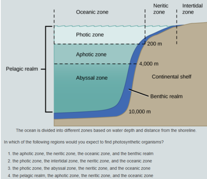
The ocean is not one uniform body of water. It is layered by light, temperature, salinity, density, oxygen and depth. Those layers decide where life can grow, where heat is stored, where oxygen is replenished and where pollution accumulates.
The first dividing line is light.
On land, light is usually available unless something temporary blocks it: cloud, smoke, dust, fog, forest canopy or weather. In the ocean, the barrier is permanent. Water itself absorbs and scatters sunlight. Near the surface, enough light remains for photosynthesis. This sunlit layer is called the photic zone. It is where phytoplankton, algae and other photosynthetic organisms can turn sunlight into biological energy.
Below that is the aphotic zone, where sunlight no longer reaches in useful amounts. Photosynthesis stops. Life still exists there, but it depends on sinking organic matter, predation, chemical energy or material transported from elsewhere.
This is why ocean depth matters so much !. The intertidal zone, the neritic zone over the continental shelf, and the sunlit part of the open ocean can all support photosynthetic life. But once water becomes too deep or too dark, biology changes completely. The ocean is not just divided horizontally by coastline and distance from land. It is divided vertically by light, and that’s where the ships are dumping their effluent, billions of litres of heavy metals and sulphuric acid.
That vertical structure is central to climate risk.
The ocean stores far more heat than the atmosphere. It heats and cools more slowly than air, and it moves that stored energy through currents, mixing, upwelling and deep-water formation. These movements help regulate weather, rainfall, storms and global temperature patterns. In marine systems, currents are not background details. They are part of the planetary engine.
Freshwater systems are often dominated by density layering: warm water over cold water, fresh water over salty water, oxygen-rich water over oxygen-poor water. Marine systems have the same problem at larger scale. When surface water warms, it becomes lighter. When freshwater enters from rain, rivers or melting ice, it also becomes lighter. That lighter surface layer can sit on top of denser water below, reducing vertical mixing.
That matters because oxygen enters the ocean mostly at the surface.
If the upper layer does not mix well with deeper water, oxygen cannot easily reach the lower layers. Meanwhile, microbes and animals continue consuming oxygen below. The result is a widening gap: the surface can look alive, even over-productive, while the water underneath is losing oxygen.
This is where shipping pollution becomes more than a surface contamination issue.
Marine engines produce sulphur oxides, nitrogen oxides, soot, metals and partially burned hydrocarbons. Exhaust gas cleaning systems, usually called scrubbers, are designed to remove part of this pollution from ship exhaust. But in open-loop systems, the pollution is not eliminated. Much of it is transferred into seawater.
Open-loop scrubbers take in large volumes of seawater, spray it through the exhaust stream, and discharge the altered washwater back into the ocean. That washwater can contain acidic compounds, sulphites, sulphates, nitrates, nitrites, polycyclic aromatic hydrocarbons, soot-associated particles, and trace metals such as vanadium, nickel, copper and lead.
The ship cleans the air by discharging effluent into the sea as a dump.
The problem is not only the chemistry. It is the geography because the ships crowd together..
Shipping lanes are repeated corridors. Ships move through the same channels, ports, straits, shelves, fjords, estuaries and coastal approaches day after day. That means scrubber discharge isnt spread evenly across the open ocean. It is concentrated along fixed industrial routes, often in waters that are already biologically active, shallow, stratified, poorly flushed or close to human runoff. Remember, these are the same routes that the sulphur was traditionally emitted, causing albedo and mirroring, so we accidentally made it hotter from the sun and easier to heat from the effluent
This creates a layered risk.
In the photic zone, added nitrogen can act as a fertiliser. In normal marine ecosystems, nitrogen often limits the growth of phytoplankton. Add enough reactive nitrogen to sunlit water and the system can be pushed toward artificial blooms. These blooms may look like productivity, but they can become the first stage of oxygen collapse.
During the active bloom phase, phytoplankton photosynthesise near the surface. They can even create high oxygen levels in the thin surface layer during daylight. But that surface signal can be deceptive. It does not mean the whole water column is healthy. It may simply mean the upper skin of the ocean is temporarily overactive while deeper layers are being set up for oxygen loss.
As we all know, blossoms do not last forever.
When the bloom exhausts available light, nutrients or trace elements, large amounts of phytoplankton die. That dead biomass sinks out of the photic zone. As it falls through the water column, bacteria begin to break it down. This decomposition requires oxygen. The more organic matter sinks, the more oxygen bacteria consume.
This is biochemical oxygen demand, or BOD.
Scrubber washwater can also create chemical oxygen demand, or COD, when reactive compounds in the effluent consume oxygen directly through chemical reactions. So the system can be hit twice: first by chemical oxygen drawdown, then by biological oxygen drawdown as bloom material sinks and decomposes.
In well-mixed open water, some of this stress may be diluted or ventilated. But in stratified systems, the deeper layers are partly cut off from the atmosphere. A thermocline, halocline or pycnocline can act like a lid. Warm, fresh or less dense water stays above. Colder, saltier or denser water remains below. Oxygen from the surface does not move downward fast enough to replace what bacteria and chemical reactions consume.
That is how bottom water loses oxygen.
Once dissolved oxygen levels fall sufficiently, benthic organisms suffer first. The benthic realm is the seafloor environment: sediments, shellfish, worms, bottom-feeding fish, microbial communities and buried organic matter. These ecosystems cannot simply swim upward and escape. When oxygen collapses near the bottom, the sediment becomes a stress zone. Fish avoid it if they can. Shellfish, larvae and bottom organisms often cannot.
This is the basic dead-zone mechanism.
The new question is whether open-loop scrubbers can help manufacture smaller, corridor-shaped versions of that process along shipping routes and port approaches.
The pathway:
Scrubber discharge adds reactive chemistry and nutrients to sunlit water.
Sunlit water can alter phytoplankton growth.
Bloom material eventually dies and sinks.
Bacteria decompose that biomass and consume oxygen.
Stratification prevents rapid oxygen replacement.
Bottom water and sediments become oxygen-stressed.
This does not require the whole ocean to become polluted. It only requires repeated discharge into the wrong physical setting: shallow shelves, fjords, estuaries, port basins, low-flushing lagoons, coastal current traps and stratified shipping corridors.
That is the model problem.
A coarse model grid can average a ship lane, a port, a stormwater outlet, a productive shelf, a deep channel and an offshore control area into one diluted box. But the ocean does not experience pollution as a grid average. The plume is local. The bloom is local. The sediment oxygen demand is local. The benthic collapse is local. The damage happens where the chemistry, biology and layering actually meet.
The sea surface may look blue from space. The average concentration may look harmless on paper. But beneath that average, the real system can contain narrow corridors of chemical stress, artificial productivity, sinking biomass and oxygen loss.
The ocean is not an infinite mixing bowl. It is a layered climate engine. The surface layer controls light, plankton, cloud-relevant biology and gas exchange. The middle layers control heat, salt, oxygen and ventilation. The seafloor records what sinks out of the system. Scrubber effluent enters at the top, but its damage can emerge below, after chemistry, biology and stratification have transformed it into oxygen demand and sediment stress. That is why planetary models must treat shipping discharge as a layered, point-source forcing, not as harmless dilution into a global average.
The Illusion of Dilution: Validating the Sub-Grid Scale Failure
The persistence of open-loop scrubber technology relies on regulatory frameworks that mathematically endorse the dilution paradigm.
Broad spatial dispersion models analysing cumulative impact over ten-year projections conclude that accumulated concentrations of nitrates, COD, and heavy metals remain orders of magnitude below ambient baseline concentrations.
Based on these averaged calculations, macroeconomic regulatory defences maintain that there is no scientific justification to prohibit open-loop discharges.
This defence is structurally compromised by the mathematical failure inherent in uniform-grid climate modelling.
Applying a grid-scale average to a highly localised, mobile point source mathematically obliterates the acute, non-linear realities of the effluent plume.
Ocean dynamics do not operate as perfectly mixed reservoirs. Sub-grid scale physical processes heavily dictate the behaviour of highly concentrated point-source discharges.
Models analysing deep-water point sources demonstrate that the vertical profile of chemical decay, sheared current strength, and local bathymetry confine toxic elements to highly localised zones that uniform coarse models fail to parameterise.
Dilution averages ignore that PAHs and heavy metals are entirely recalcitrant. They persist and bioaccumulate rapidly through the zooplankton boundary layer upward into apex taxa, regardless of initial volumetric dilution.
A projected minimal pH drop across a large bay is a statistical artifact that ignores the continuous, highly acidic physical wake trailing a bulk carrier. Resolving the magnitude of this industrial deoxygenation vector requires high-resolution estuarine-shelf models capable of tracking dynamics down to the 7-10 km scale, isolating point-source inputs, and tracking the biological BOD responses they trigger.
Synthesis of Findings
The integration of exhaust gas cleaning systems into the global maritime fleet establishes a transfer vector for severe chemical pollutants directly into the upper ocean pelagic zone.
The unmitigated discharge of open-loop washwater inflicts acute physicochemical trauma upon the receiving environment, defined by extreme acidification, depleted carbonate buffering capacity, and the immediate introduction of recalcitrant polycyclic aromatic hydrocarbons and trace heavy metals.
Scrubber-induced environmental degradation is biphasic. An intense abiotic Chemical Oxygen Demand aggressively scavenges dissolved oxygen upon discharge. A biological cascade follows, as reactive nitrogen artificially fertilises the stratified photic zone, triggering localised phytoplankton blooms. The senescence and sinking of this biomass fuels aggressive aerobic bacterial remineralisation, resulting in severe Biochemical Oxygen Demand collapse and the formation of hypoxic dead zones directly beneath shipping corridors.
Standard Earth System Models and regulatory impact assessments systematically underestimate this localised deoxygenation vector. Uniform grid-averaging mathematically dilutes the reality of mobile, high-density point sources. The physical, chemical, and biological evidence demonstrates that marine scrubbers engineer intense, sub-grid-scale biogeochemical disruptions that threaten pelagic and benthic marine ecosystems along critical maritime transit routes.
When you view the global maps of the shipping channels, the phytoplankton distribution
Compound tails, CDR, and the fiction of smooth control
Compound correlated tails. The framework under-tests stacked bad outcomes. ScenarioMIP is a small suite by design. That makes it manageable, but it also means the really dangerous cases are mostly absent: stronger aerosol masking than assumed, faster aerosol unmasking, higher climate sensitivity, weaker ocean carbon uptake, AMOC destabilisation, marine productivity losses, and CDR under-delivery arriving together. AR6 WG1 says compound events and concurrent extremes increase the probability of low-likelihood, high-impact outcomes and become more frequent with warming.
The implication is that one-factor sensitivity tests are not enough. Tail-risk work needs coherent bad-combination pathways.
CDR and overshoot control. Claim: The framework assumes too much future control. The paper’s long extensions are all designed to achieve temperature stabilisation after 2300.
All extensions except Very Low reach net-zero CO₂ by 2300; the High extension reaches net zero by 2250; and the more extreme overshoot extensions require prolonged net removals reaching roughly −9, −11, and −22 GtCO₂ yr⁻¹ in the mid-22nd century. At the same time, the paper admits that most ESMs are not yet ready to simulate BECCS directly, so BECCS carbon storage and net emissions are passed from IAMs to ESMs rather than being computed fully within them.
The implication is that overshoot and reversibility are being explored under a stylised assumption of eventual control, not under contested real-world deployment constraints.
CDR feasibility. The literature does not support casual confidence in that late control. AR6 WGIII says pathways limiting warming to 2°C or lower involve some CDR, but it also says that AFOLU sinks ultimately saturate, that large-scale land-based CDR can damage biodiversity, and that stronger demand-side mitigation reduces dependence on CDR.
A 2024 Communications Earth & Environment study found that storage durations below 1000 years are insufficient to neutralise residual fossil CO₂ under net zero, and that with 6 GtCO₂ yr⁻¹ of residual emissions, a 100-year storage duration adds about 0.8°C of warming by 2500 relative to permanent storage.
A 2025 Nature study then estimated a prudent planetary limit for geologic carbon storage of about 1,460 GtCO₂, far below many headline technical-capacity numbers.
The implication: ScenarioMIP’s overshoot cases should include explicit CDR-failure variants, not just removal pathways.
Climate-impact feedbacks. Claim: the framework excludes a major amplifier. The paper says IAM teams should not include climate change impacts on agriculture, energy use, economic growth, or biodiversity, and later says that versions with climate impacts should be developed in future. It also says adaptation-mitigation interactions are not currently considered.
The implication is that the socio-economic side of the scenarios stays too orderly under severe warming. That is logically misleading, as it occurs exactly where upper-tail risk is highest, because damages can feed back into energy demand, food systems, migration, fiscal capacity, conflict risk, and the ability to deploy mitigation and CDR.
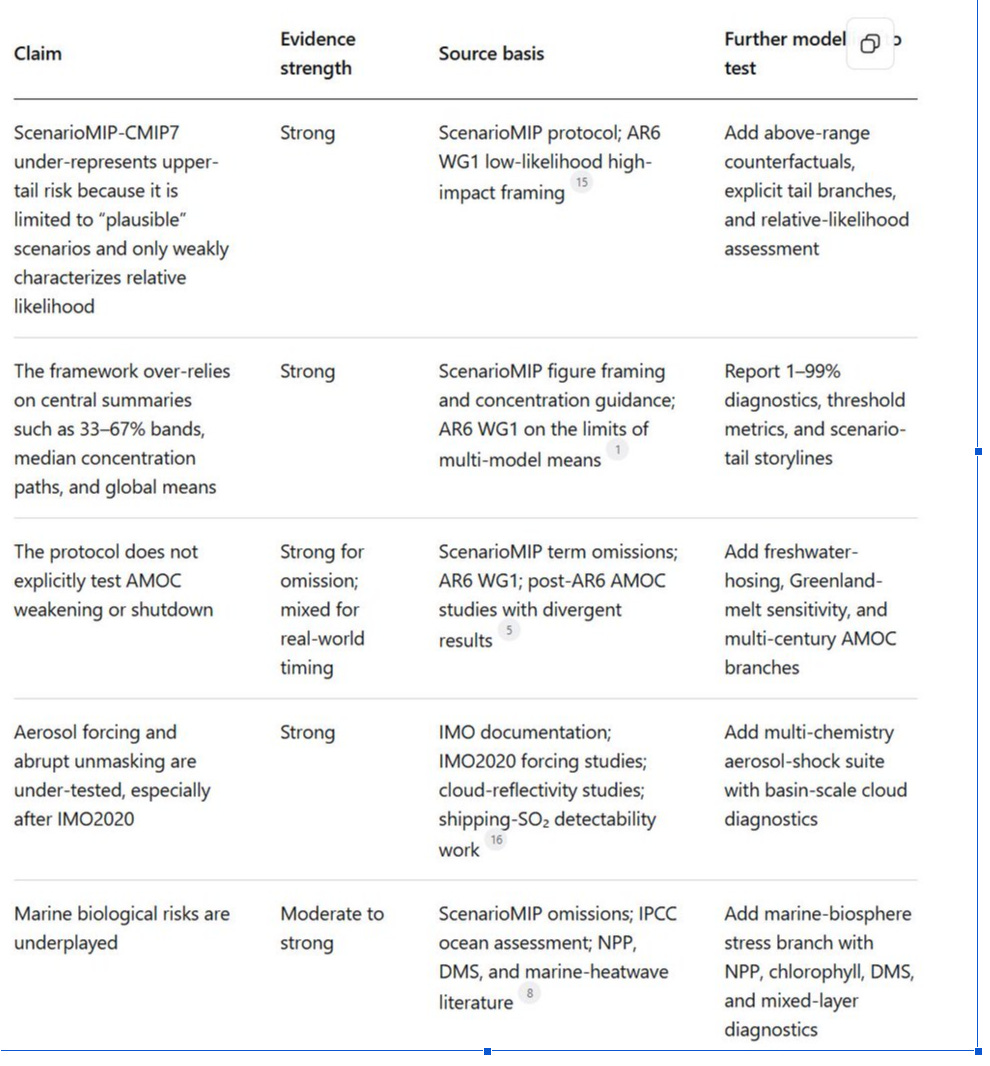
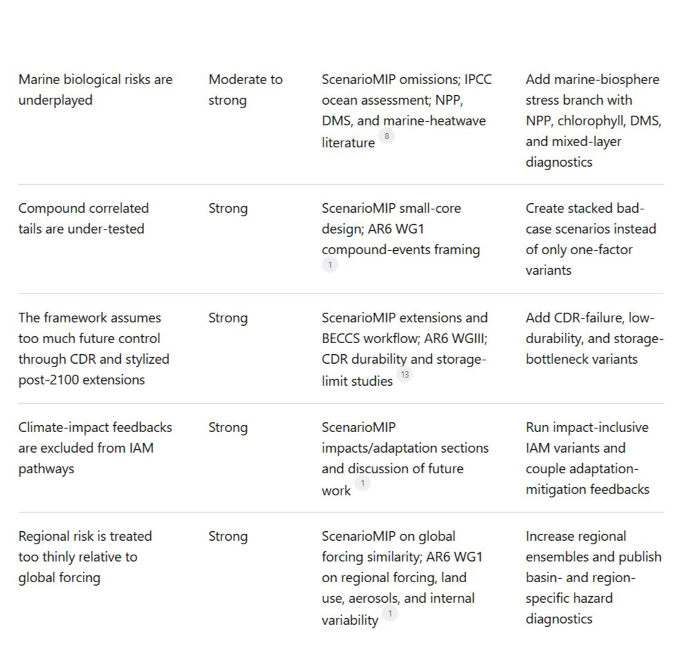
Claims and their tests for Easy Reference
A Novel Addition to Climate Risk
The unique claim of this paper is that modern ocean-circulation risk is being assessed without fully accounting for the industrial surface-ocean layer now sitting on top of circulation-sensitive regions.
AMOC, ENSO, Mediterranean outflow, upwelling systems and oxygen-minimum zones are usually studied through physical climate variables: temperature, salinity, winds, freshwater, stratification and radiative forcing.
But the modern ocean also contains concentrated maritime and coastal chemical forcing: scrubber effluent, tyre-wear particles, road runoff, PAHs, metals, synthetic additives, black carbon, altered aerosols and biological sulphur disruption.
These inputs are not evenly distributed. They cluster around ports, shipping lanes, estuaries, chokepoints and productive coastal waters. The novelty lies in the coupling: the same regions that regulate heat, salt, oxygen, clouds, and biological productivity are increasingly exposed to no-analogue industrial stress. The question is no longer whether each mechanism matters in isolation. The question is whether their overlap creates acceleration pathways that existing models, paleoclimate analogues and scenario frameworks are structurally prone to miss.
In this diagram, I have isolated how the multiple systems overlay each other
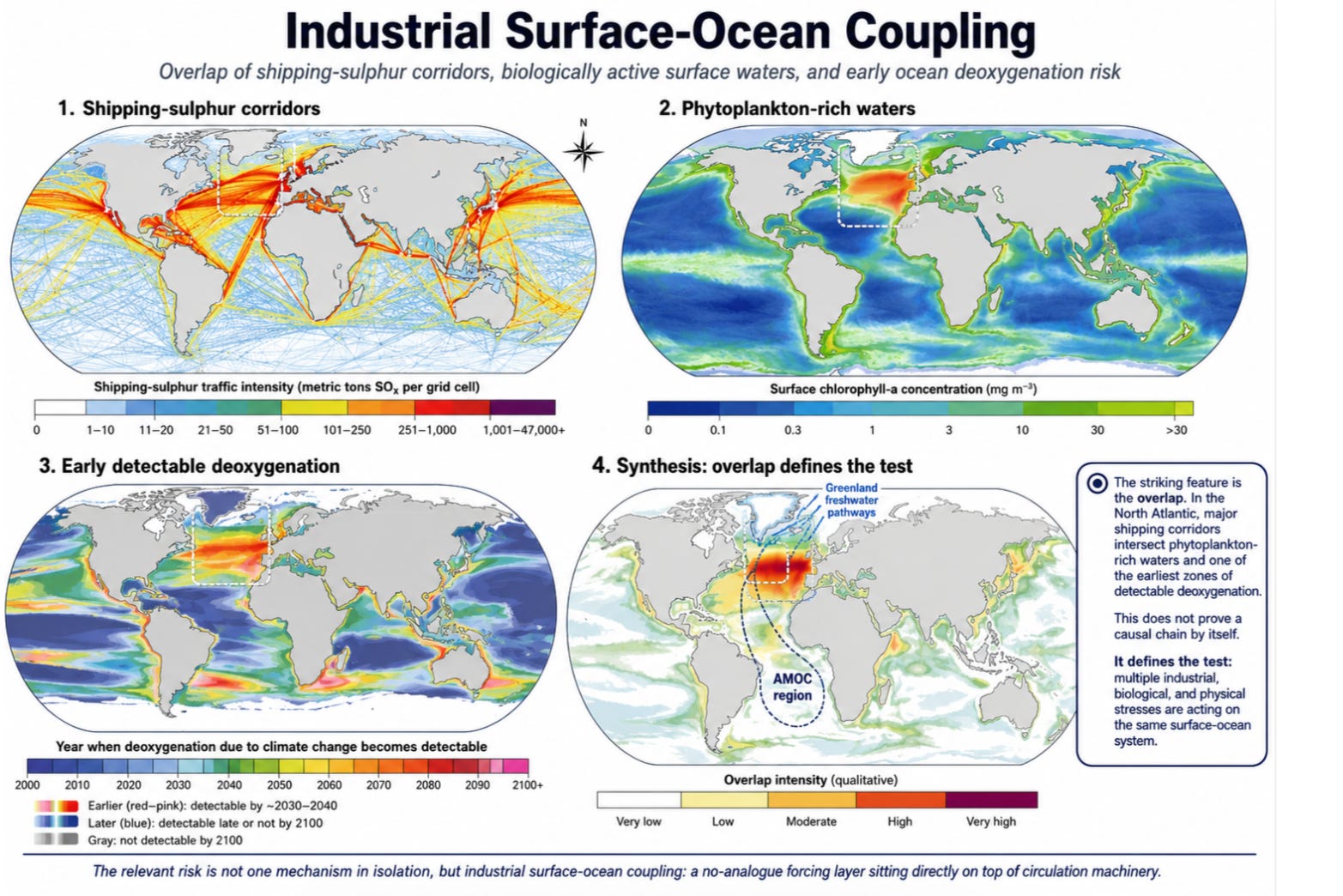
The striking feature of the global maps is not any single layer. It is the overlap. Historic shipping-sulphur corridors trace the fixed industrial arteries of the ocean. Phytoplankton maps show where the surface ocean is biologically active enough to shape carbon cycling, cloud chemistry, light absorption and food-web stability. Deoxygenation maps show where warming and stratification are expected to make oxygen loss detectable first.
When these layers are placed side by side, the coincidence isn’t random-looking. It is especially suggestive in the North Atlantic, where major shipping corridors intersect with phytoplankton-rich waters, aerosol-sensitive cloud regimes, likely Open Loop scrubber discharge , Greenland freshwater pathways and the broader AMOC system.
If the same ocean surface is being aerosol-altered from above, chemically loaded from ships and runoff, biologically stressed through phytoplankton and DMS pathways, and physically freshened by meltwater, then the relevant risk is not one mechanism in isolation. It is industrial surface-ocean coupling: a no-analogue forcing layer sitting directly on top of circulation machinery.
The paleoclimate record is often used as a guide to AMOC risk, but it may be an incomplete guide to the present.
Earth history contains freshwater-forced overturning disruptions, including events associated with abrupt North Atlantic climate shifts, but it of course does not contain the modern industrial forcing stack now acting on the same system.
The present North Atlantic is being stressed simultaneously from above, below and within: greenhouse warming raises the ocean heat baseline; Greenland meltwater freshens and stratifies the surface; post-2020 sulphur reductions weaken part of the aerosol-cloud cooling mask; marine cloud reflectivity has declined across key North Atlantic and Northeast Pacific regimes; phytoplankton and DMS pathways may alter cloud-condensation and light-absorption dynamics; and scrubber effluent, tyre runoff and port pollution add toxic, oxygen-demanding chemical loads to coastal and shipping-lane waters. None of these mechanisms alone proves imminent AMOC shutdown.
The danger is that they are usually assessed separately, while the physical ocean receives them together. If these pressures reinforce one another, the pathway to Atlantic overturning failure may be much faster, more localised and less visible in ensemble means than paleoclimate analogues or coarse-grid models imply.
The Earth record shows that the trapdoor exists. It may not show what happens when modern industrial society pushes on that trapdoor from five directions at once.
Another expression of this thesis is El Niño, a basin-scale Pacific mode driven by ocean heat recharge, wind anomalies, Kelvin waves, thermocline shifts, and coupled ocean-atmosphere feedbacks. But let’s consider how it is impacted by modern industrial forcing.
The Panama Bight and nearby shipping corridors lie within a sensitive ENSO expression zone, where El Niño already raises SST and sea level, weakens upwelling, and alters biological conditions.
That region is also exposed to intense shipping, port activity, scrubber discharge risk, tyre and road runoff, atmospheric deposition and post-2020 aerosol-cloud disruption. The hypothesis is therefore not that Panama “causes” El Niño.
Modern El Niño events now pass through a no-analogue coastal amplification layer: higher background heat, reduced sulphur-driven cloud brightening, altered phytoplankton and DMS pathways, pollution-driven biological stress, and weaker local buffering.
This could make eastern Pacific El Niño expression hotter, more persistent or more biologically damaging than historical analogues imply, even if the basin-scale ENSO trigger remains unchanged. It’s just common sense.
It’s common sense that the paleorecord contains El Niño, it’s just as sensible that the record doesn’t contain El Niño running through a modern eastern Pacific corridor of greenhouse heat, post-IMO aerosol unmasking, dense shipping, scrubber effluent, tyre runoff, altered phytoplankton and synthetic chemical stress.
This is a conundrum for climate scientists, especially for deniers. We can’t ignore the paleo record, but we must all realise that its analogue is limited. It’s certainly a map, but it’s an old one, and modern civilisation swapped out the territory. Paleo Record Fixation (PRF) should be described as an intellectual condition
X Readers start here
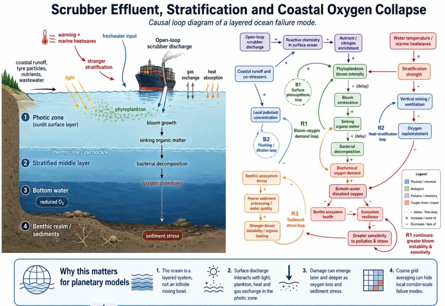
What a real tail-risk protocol would add
The fix is not mysterious. It is mostly a matter of admitting what the current protocol is for, and then adding the pieces it does not try to do.
First, ScenarioMIP should add explicit AMOC branches: freshwater-hosing experiments, spatially realistic Greenland-melt sensitivity experiments, and more 2300–2500 runs than just the preferred extensions. The entire point is to stop leaving AMOC collapse or severe weakening as an accidental model by-product.
Second, it should add an aerosol-shock suite: multiple chemistry realisations, explicit IMO2020-style abrupt-unmasking branches, and basin-scale diagnostics of marine cloud reflectivity over the North Atlantic and Northeast Pacific. The protocol already admits that one chemistry model is too narrow. It should act on that admission.
Third, it should add a marine-biosphere stress branch: stronger-stratification cases, weaker NPP cases, DMS-suppression cases, and mandatory reporting of chlorophyll, mixed-layer depth, deep chlorophyll maxima, and marine heatwave impacts. The climate system is not just radiation, carbon, and circulation. It is biology, too.
Fourth, it should include CDR-failure variants: delayed scale-up, reduced durability, storage bottlenecks, land-use conflicts, and higher residual emissions. Overshoot scenarios should not be allowed to look clean just because removals are scripted.
Fifth, it should add impact-inclusive IAM pathways and correlated-tail scenarios. The paper itself recommends scenarios with climate impacts and says relative likelihoods need more work. That future work should not be optional. It should be inside the protocol for any framework that claims to inform risk.
Finally, it should stop centering the middle of the distribution. The standard package should report 1–99% diagnostics, threshold indicators, single-model large ensembles for regional extremes, and regional hazard outcomes rather than mostly global means. AR6 already explains why.
The hard conclusion is this: ScenarioMIP-CMIP7 is a good intercomparison design and a weak upper-tail risk protocol. The problem is not dishonesty. The problem is that a tractable, plausible, globally averaged experiment design gets mistaken for a full map of danger. It is not. The high-tail climate risk sits in the parts that plausibility filters, medians, multi-model means, and stylised reversibility smooth away.
The Consensus Machine
When model architecture becomes institutional architecture
Until this point, the argument has been about the architecture of climate modelling.
Uniform freshwater hosing can make a sharp AMOC risk look gradual. Relative ENSO indices can remove absolute heat from the risk ledger. Central Scenario MIP summaries can make tail risk look narrower than it is. Global averages can flatten regional shocks. Plausibility filters can exclude the very futures a risk system should be stress-testing.
But wait, there is more: another layer.
The modelling architecture is not the only place where risk gets smoothed. The IPCC institutional architecture does it too. It passes through a chain of selection, modelling, assessment, negotiation, compression and amplification. By the time a finding appears in a public-facing IPCC summary, it has already travelled through scenario choices, model infrastructure, assessment conventions, expert networks, government negotiations, and institutional incentives.
Climate authority is institutionally processed. The processing can make dangerous, uncertain, politically uncomfortable risks appear cleaner, slower, smoother and more settled than they really are.
It is the final public-facing compression layer of a much larger machine.
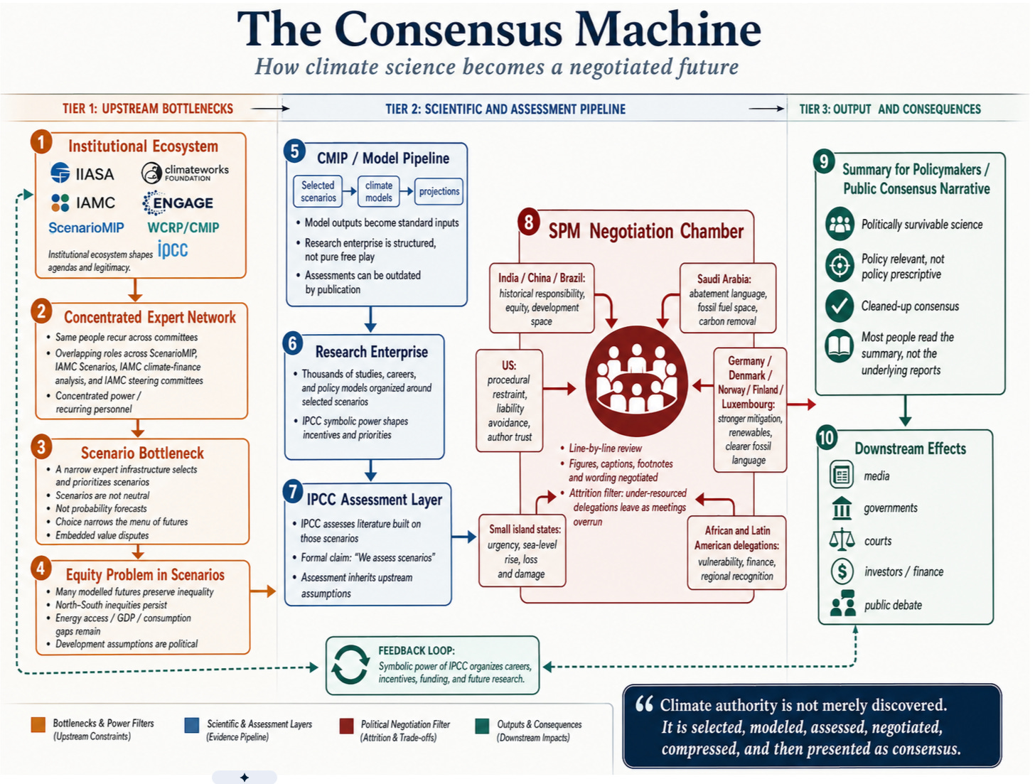
The Consensus Machine. This systems-flow map shows how climate authority moves from upstream scenario selection and institutional bottlenecks through model pipelines, IPCC assessment, Summary for Policymakers negotiations, and downstream public consensus. The orange tier shows upstream power filters; the blue tier shows the scientific and assessment pipeline; the red tier shows the diplomatic negotiation filter; and the green tier shows public outputs and consequences. The country boxes illustrate recurring pressure points during the IPCC-58 negotiations, not permanent national positions. The dashed feedback loop shows how IPCC authority can organise careers, funding, institutional priorities and future research agendas.
The Model of the Model of the Model
Climate science begins with an unavoidable modelling problem. The Earth system is too complex to reproduce directly, so climate scientists use models, ensembles, scenarios, parameterisations, confidence language, and emissions pathways. That does not make the science useless. It means the science is mediated. What I will outline here is how the models are processed by technocratic bureaucracy.
Then comes the second layer: model comparison. The Coupled Model Intercomparison Project, or CMIP, is a project of the World Climate Research Programme. It coordinates model experiments and has become essential to IPCC and other climate assessments. CMIP describes its multi-model approach as a way to evaluate models, improve simulations, and understand past, present, and future climates.
Then comes the third layer: scenario selection. ScenarioMIP carries out Earth-system model simulations driven by alternative plausible futures of emissions and land use. It explicitly integrates climate science, integrated assessment modelling, mitigation research, and impacts/adaptation/vulnerability communities.
Then comes the fourth layer: the IPCC assesses literature built on those model outputs and scenario frameworks.
Then comes the fifth layer: the Summary for Policymakers compresses the assessment.
Then comes the sixth layer: governments approve that summary line by line.
So the public does not receive “climate science” as raw discovery. It receives the end product of a long chain:
Earth system → scenarios → models → model comparisons → assessment literature → IPCC synthesis → Summary for Policymakers → government approval → public consensus narrative
Every arrow is a compression event. Every compression event changes something. What gets removed is not always the truth. Often, it is context, uncertainty, disagreement, value conflicts, tail risk, political asymmetry, and the visibility of upstream choices. That is why the phrase “scientific consensus” can be misleading. Consensus is produced by a process of discussion, and how it is produced is a model in itself
The Gap in Conventional Risk Assessment
Earth’s climate is a complex, coupled system with feedbacks, delays, thresholds, and abrupt shifts. Standard frameworks often treat it as approximately linear. Recent evidence confirms the mismatch.
A 2026 Science Advances study using observational constraints (temperature, salinity, and ridge-regularised regression) projects 51 ± 8% AMOC weakening by 2100 under medium-to-high emissions—approximately 60% stronger than CMIP6 multi-model means (~32%). This level of slowdown is “almost certain to end in collapse” once a tipping threshold is crossed, with committed weakening possible within the next 10–30 years under continued forcing. science.org
James Hansen and colleagues (2025–2026) document a sharp decline in planetary albedo (based on CERES data), driven largely by reduced anthropogenic aerosols, including post-IMO 2020 shipping sulphur cuts, combined with positive cloud feedbacks. This has amplified Earth’s energy imbalance (~1.5 W/m² in recent periods) and supports an effective climate sensitivity of 4–5°C per CO₂ doubling (far above IPCC’s 3°C best estimate). jimehansen.substack.com
Ocean biology compounds the issue: declining chlorophyll and net primary productivity in low-to-mid latitudes, driven by stratification and warming, reduce dimethyl sulphide (DMS) production and cloud-seeding, enabling deeper solar heat penetration and further albedo loss.ScenarioMIP-CMIP7 improves long-term runs but retains core limitations: plausibility filters, central summaries, single-chemistry aerosol realisations, and limited explicit treatment of realistic hosing, marine biosphere feedbacks, or impact-inclusive pathways.
The Coupled Earth System Risk Protocol ()
The CESRP reframes the core question:
“Is the mechanism physically plausible? Are signals aligning? Would it delay close response windows? Do coupled tails threaten systemic failure?”
Five Operational Pillars 1. Physical Plausibility & Mechanism Mapping
Score mechanisms 1–5 using process understanding, paleoclimate, and high-resolution experiments:
Point-source Greenland meltwater into fjords creates sharp buoyancy anomalies and salt-advection feedback (Score: 5).
Aerosol unmasking + phytoplankton/DMS decline → deeper heat absorption + albedo loss (Score: 4–5).
2. Observational Signal Directionality
Prioritize vectors: RAPID array weakening, CERES albedo drop (~0.62 points), absolute ocean heat content, chlorophyll declines, and polar motion from mass redistribution. Use absolute thermal stress alongside relative indices.
3. Reversibility Window & Commitment Analysis
Quantify time-to-threshold vs. time-to-response. Observational constraints indicate committed AMOC weakening within 10–30 years; full shutdown becomes a serious tail risk thereafter. Aerosol acceleration and biological feedbacks shorten windows. Irreversible elements (major ice loss, regime shifts) demand pre-threshold action.
4. Compound Tail Stress Testing (New Quantitative Bounding)
Explicitly model or bound correlated high-impact scenarios:
Realistic-topography AMOC hosing + IMO-style aerosol unmasking + phytoplankton/DMS suppression + deeper heat uptake.
AMOC collapse alone could release stored ocean carbon, adding 0.17–0.27°C extra global warming over centuries. Combined feedbacks (albedo + biology + carbon cycle) plausibly amplify total warming by an additional 0.3–0.6°C by 2100 beyond central projections.
These tails raise the effective Social Cost of Carbon to $250–350+ per ton CO₂ (vs. many published averages of ~$130–190), when omitted channels and fat-tail risks are included. pik-potsdam.de +1
Output: Full risk envelopes (1–99th percentiles, threshold probabilities) rather than medians.Methods Box: Risk Urgency Index (RUI) Scoring (0–100)
Pillar 1 (Plausibility): ×20
Pillar 2 (Signals): ×20
Pillar 3 (Window): ×25 (heavier weight on closing windows)
Pillar 4 (Tails): ×25
Pillar 5 (Brittleness): ×10
Interpretation:
0–40: Enhanced monitoring.
41–70: Accelerated mitigation + resilience.
71–100: Emergency-scale response, including research into all options under strict governance.
5. Systemic Failure Mode & Brittleness Assessment
Map how food systems, insurance, ports, grids, and migration break under nonlinear shifts. Stress-test “what if the mean never occurs?”Implementation Recommendations (2026–2030)
Research: Require realistic point-source hosing, multi-realisation aerosol suites, marine biosphere diagnostics, and compound-tail ensembles in CMIP8.
Policy & Finance: Embed CESRP in national risk registers, central bank stress tests, and insurance models. Price emissions at tail-informed levels as clean energy scales.
Communication: Reframe public discourse around safe operating space and physical mechanisms.
From Map to Compass, models are essential maps, but they aren’t the territory. The 2026 evidence, 51% projected AMOC weakening, record albedo decline, biological feedbacks—shows signals aligning with high-plausibility coupled risks. Waiting for ensemble consensus risks closing critical windows.
The CESRP operationalises the “castle lookout” standard into a repeatable, quantified protocol suited to nonlinear reality.
It is not alarmism; it’s just a better system thinking, it is rigorous, systems-aware prudence at the planetary scale. Implementing it now in research agendas and decision frameworks is essential.
Selected References
Portmann et al. (2026). Observational constraints project ~50% AMOC weakening. Science Advances.
Hansen et al. (2025–2026). Acceleration, cloud feedback, and high sensitivity papers.
Nian et al. (2026). AMOC collapse carbon release (~0.2°C).
Expert syntheses on elevated SCC under tails.
The Calculus of Physical Ruin: Industrial Coupling and the Open-Loop Protocol
I. The Architecture of Collapse
Earth’s climate is a complex, coupled system operating with feedbacks, delays, thresholds, and abrupt shifts. Standard risk models process this physical reality through mathematical dilution, compressing extreme, localised processes into parameterised rules and grid-cell averages.
This informational architectural failure masks the mechanisms driving planetary instability. The true danger resides in the sub-grid scale. Industrial shipping networks continuously inject severe chemical, biological, and thermal disruptions directly into the ocean’s layered circulation systems.
Shipping-sulphur corridors, phytoplankton-rich waters, and early deoxygenation zones overlap geographically.
This creates industrial surface-ocean coupling: a synthetic industrial forcing layer superimposed directly upon primary oceanic circulation machinery. This establishes compounded stressors completely absent from paleoclimate analogues.
Albedo Degradation: The reduction of marine sulphur aerosols eliminated a primary source of cloud condensation nuclei, initiating an abrupt decline in planetary albedo. Earth currently absorbs an additional $2.09~W/m^{2}$ of solar energy. Thermal stress and freshwater stratification suppress phytoplankton populations, breaking their biological cloud-seeding mechanism. This enables deeper penetration of solar heat and further albedo degradation.
Biphasic Oxygen Collapse: Open-loop scrubber effluent drives a severe physicochemical transformation of the water column. The discharge creates an intense abiotic Chemical Oxygen Demand spike. The effluent’s reactive nitrogen subsequently fertilizes the surface layer, triggering rapid phytoplankton blooms. The subsequent senescence and sinking of this biomass fuel aggressive bacterial respiration in deeper, stratified waters, exhausting dissolved oxygen and causing severe hypoxic zones. Hydrodynamic constraints and density-driven stratification trap this concentrated toxic effluent within the photic zone along fixed commercial shipping corridors.
Circulation Failure: Standard Earth System Models distribute Greenland meltwater evenly across massive oceanic grids, mathematically misrepresenting heterogeneous melting patterns. Injecting freshwater at specific localized coordinates forces the modelled AMOC to react to concentrated pockets of extreme buoyancy, resulting in sudden, steep circulation declines of 20%.
II. The Consensus Machine
The institutional architecture of climate science operates as a consensus machine. Plausibility filters, multi-model means, and political negotiation structurally engineer this consensus. This sequential compression systematically erases the visibility of low-likelihood, high-impact regional thresholds before the data reaches public-facing summaries.
Utilising relative tools obscures the total absolute heat entering the biosphere. Ecosystems, infrastructure, and agricultural supply chains respond to absolute heat stress. Demanding perfect proof from these compromised models operates as an independent vector of systemic risk.
In many ways, the research publication model needs to accelerate the scale of the challenge,
III. The Corrective Framework
Calculating the timeline to an irreversible threshold demands action before the viable response window closes. The Coupled Earth System Risk Protocol (CESRP) establishes an operational framework for systemic risk management by integrating physical plausibility, observational signal directionality, and compound-tail stress testing.
Open Loop Intellectualism (OLI) operationalises this protocol. It distributes analytical models directly into the public domain for continuous modification, structural expansion, and collective stress-testing. This operates as a live, interactive programming interface for human cognition. The expert group transitions into a strict validation node and executes a compiler function. Incoming causal loops and localised datasets merge into the active baseline exclusively upon satisfying the physical and mathematical constraints of the CESRP.
Compilers are expert gatekeeper communities. The idea is not to destroy the expert layer but to flatten it intelligently to accelerate productivity.
IV. The Material Capital Engine
The financial architecture isolates the compiler node from legacy capital. Traditional finance defends the illusion of aqueous dilution to protect existing liability pricing. Funding requires extracting capital directly from entities dependent on physical reality.
The Industrial Counterpart Bond: Large-scale industrial debt covenants require an absolute oracle to verify physical metrics, thermal inputs, and material output. The compiler node serves as this exclusive clearinghouse, mathematically locking operational funding into the debt structure.
The Material Ledger Arbitrage: Hard-asset allocators and tier-one supply chain operators require the exact physical coordinates of systemic failure to survive structural de-industrialisation. Restricting the live feed of the CESRP risk matrix to a subscription architecture forces capital allocators to fund the intelligence node to front-run the collapse of grid-averaged forecasting.
Let me highlight that the above is just a suggestion. There are many ways of doing this its part of re-architecting capitalism to be more functional and successful.
Validated data deploys directly into an indexed Information Cube. This archive operates as the primary distribution node for industrial systems intelligence. Operators ingest this data, adjust physical positions, and generate new systemic pressures that feed back into the compiler’s direct ingestion layer for automated stress testing.
A New Type of Climate Science
The architecture of ocean mechanics operates as a computationally irreducible system. Earth System Models simulate marine dynamics through continuous mathematical dilution, applying uniform grid-averaging to calculate scalar shifts in salinity and temperature.
This methodology distributes localised chemical and thermal inputs evenly across vast aquatic surface areas. Physical reality executes through discrete, localised, geometric interactions.
The global maritime fleet functions as a macro-scale execution of mobile automata. Standard models evaluate point-source emissions as static variables. A bulk carrier utilising an open-loop scrubber operates as a singular active cell moving along a fixed geometric corridor.
The vessel actively alters its immediate grid cell, discharging highly concentrated unoxidized sulphur compounds and reactive nitrogen directly into the photic zone. The resulting spike in Chemical Oxygen Demand initiates a sequential substitution system within the biological architecture of the water column. It sorts itself out according to rules.
The sequence executes deterministically: reactive nitrogen replaces the baseline nutrient state. This parameter initialises a rapid phytoplankton bloom. The biomass exhausts available light, initiating senescence and substituting the living bloom with sinking organic matter. Heterotrophic bacterioplankton consume this substrate, thereby increasing the organic material’s severe Biochemical Oxygen Demand and localised hypoxia.
The thermocline and halocline establish impenetrable physical boundaries formed by temperature and salinity differentials. This geometric confinement restricts the substitution system to the stratified surface layer, forcing the algorithm to iterate rapidly upon itself within the shipping corridor.
Evaluating this coupled system requires models that execute localised, step-by-step algorithms. Analysis of cellular automaton Rule 110 demonstrates that simple, localised rules generate immense, irreducible complexity. The ocean produces analogous localised structures: migrating hypoxic dead zones, restricted albedo degradation, and isolated thermal stratification.
AMOC responds directly to the mass geometry produced by this coupled ice-ocean-water system. Injecting freshwater at specific localised coordinates forces the system to process acute density drops, resulting in immediate, steep declines in circulation.
The Coupled Earth System Risk Protocol establishes the necessary computational framework. The protocol forces the calculation of compound-tail stress tests and localised mechanisms.
Open Loop Intellectualism distributes analytical models directly into the public domain for continuous structural expansion. Capital allocators and industrial operators must fund this intelligence node to determine the exact physical coordinates of systemic failure. Validated data deploys directly into the Information Cube, functioning as the primary distribution node for industrial systems intelligence. The compiler node ensures the calculation of the mechanical progression of ocean deoxygenation governed exclusively by physical and mathematical constraints.
Why this matters
The issue is that models and indices are built for specific purposes. A tool designed to estimate broad averages may miss shocks. A tool designed to identify weather-pattern contrast may not measure total heat stress. A hosing experiment that spreads freshwater evenly may not capture what happens when meltwater enters through narrow coastal pathways.
Averages make a sharp physical risk look smoother than are.
That does not mean every alarming scenario is true. It means the standard for action has to match the system being assessed.
For a slow and reversible problem, waiting for full certainty can make sense.
For a linked climate system with long delays and serious downside, waiting for perfect proof can become its own risk.
The better standard is:
Is there a clear physical mechanism?
Are observations moving in the wrong direction?
Could delay make the outcome harder to reverse?
Are the consequences large enough to justify early action?
That is not alarmism. It is basic risk management.
The climate system does not need to become uninhabitable to create severe human problems. Modern food systems, water systems, insurance markets, ports, power grids, migration patterns, and public finances were built inside a fairly stable climate envelope.
Move far enough outside that envelope, and systems can become brittle.
The Younger Dryas is a useful reminder that abrupt climate shifts are part of Earth’s history. It began around 12,900 years ago, lasted roughly 1,200 years, and included abrupt temperature changes in parts of the Northern Hemisphere. The point is not that the present will repeat the Younger Dryas. The point is simpler: abrupt climate change is real, and Earth systems do not always move gradually.
So the argument should be clear and grounded:
Climate risk is not only about the average warming trend. It is also about feedbacks, thresholds, regional shocks, and linked systems moving together.
A model average can be technically useful yet miss the shape of the danger.
That is the mismatch.
We are trying to assess a nonlinear Earth system with habits built for cleaner, slower, more reversible problems. The response should not be reckless. But it also should not wait until every model agrees, every mechanism is settled, and every institution feels comfortable saying the quiet part out loud.
The lookout does not wait for eye colour.
He raises the alarm when movement, speed, direction, and distance suggest the gate may be at risk.
That is the standard climate risk now required.
Ive always had a problem with the “climate change” crowd as every hurricane, storm, El Niño etc all of a sudden was “climate change”. Here in the US, anyone who has traveled the western US states with truly open eyes can see that the landscape tells a story of vastly different climate(s) throughout history.
Policy is of ten knee-jerk and political v rational and focused. Here in the US, there are great areas that work exceptionally well for solar (I’ll be adding an off grid system to my on grid home this fall as a redundancy) like CA/NM/AZ/TX etc, and there are places like the far NE states where solar is simply uneconomical. Instead of incentives to go solar wherever works best, we get a hodge podge of policies that change with succeeding administrations. In the PacNW hydro is a huge contributor, but even there they use a broad mix of energy including solar, wind, natural gas gas, etc.
Long ago the “greenies” hamstrung more nuclear in the US. Germany went beyond and literally destroyed fully functional nuke plants. That’s not smart thinking or planning, that’s a Luddite religion at work.
Many western nations outsourced their manufacturing to China, and here in the states California, a literal energy island, has seriously curtailed any oil drilling while driving refineries to shut down via onerous fines. The governor claims it’s making CA more “green”, while in reality it’s exposing CA to massive fuel shortages as now petroleum products that could be refined there, under far better standards than Asia, are instead coming in by tankers belching bunker oil smoke as they cross the Pacific. A wholly non-sensible approach overall. Not to mention exposing one of the world’s largest economies to potential foreign fickle exports.
Beyond this, while the west claims this greater “green” approach, there is little that can be done as regards pollution from China, Mexico, or other emerging economies — all affecting “climate change”.
The easiest and cheapest transport in an emerging economy like India is a motor scooter, and they come with zero emissions controls. And the Chinese build a coal fired power plant like every day practically. We know their environmental standards make 1950’s America look environmentally conscious.
There will be no change without a concerted world approach. Germany can shoot itself in the foot by shutting down nuclear (and yes this is being reversed) because they elect fools. The NE states will never be able to survive off solar, and they should not be cajoled into trying. The SW states should be given every incentive to build (individually on homes) solar as much as possible to free up what the NE (and other parts) need.
This applies around the world. Just as you note the grid approach to climate models, we need a grid approach to renewables worldwide. NOT so much because of flawed climate models, but because it’s the right thing to do. And countries such as China, India et al should also be enticed to follow the same plan.
I don’t believe any of us can know what will transpire within our lifetimes, or those or our children, with any certainty. The only we can agree upon is one day fossil fuels will become very dear, and fallback systems need to be in place before then. We are going to need buy in from around the world to make this happen.
And no, I have no personal plans to give up my diesel pickup anytime is the near future, while at the same time I expect that day to come. In the mean time solar will become a part of my life soon because it WORKS where I live. And that’s a good enough start for me.